From the free course AP Calculus AB on Lykke
7.9 Logistic Models with Differential Equations (BC only)
Key concepts: Logistic models with differential equations · Exponential growth and decay · Solution curves of differential equations · General solutions and constants of integration · Particular solutions from initial conditions · Carrying capacity and asymptotic behavior · Interpreting the meaning of a differential equation · Developing mathematical models from differential equations · The equation dy/dt = ky · BC-only calculus content
A population can grow rapidly when resources are abundant, yet slow down as food, space, or energy becomes scarce. A logistic model captures both effects by making the growth rate depend on the population’s current size and its distance from a maximum sustainable level, called the carrying capacity.
7.9 Logistic Models with Differential Equations (BC only)
A population can grow rapidly when resources are abundant, yet slow down as food, space, or energy becomes scarce. A logistic model captures both effects by making the growth rate depend on the population’s current size and its distance from a maximum sustainable level, called the carrying capacity.
BC-only scope: Logistic models with differential equations are required for AP Calculus BC, not AP Calculus AB.
The governing enduring understanding is FUN-7: “Solving differential equations allows us to determine functions and develop models.” The learning objective is FUN-7.H: “Interpret the meaning of the logistic growth model in context. BC ONLY.” The essential knowledge identifiers for this topic are FUN-7.H.1, FUN-7.H.2, and FUN-7.H.3.
The logistic differential equation
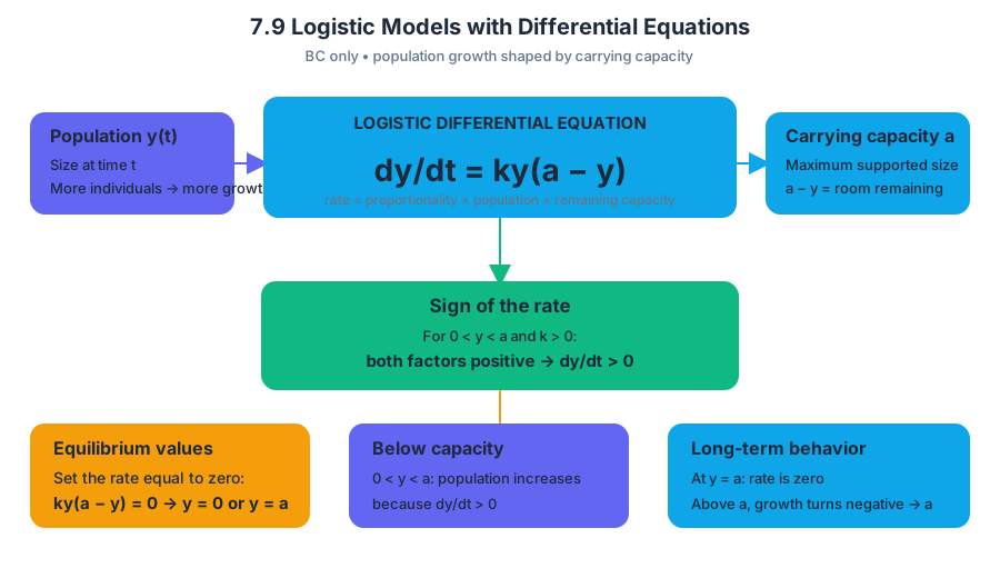
Suppose $y(t)$ represents the size of a population at time $t$, and $a$ represents its carrying capacity. The statement “the rate of change is jointly proportional to the size of the quantity and the difference between the quantity and the carrying capacity” produces the logistic differential equation
$$ \frac{dy}{dt}=ky(a-y). $$
Here, $k$ is a proportionality constant. The factor $y$ means that a larger population can produce more offspring or otherwise generate more growth. The factor $a-y$ measures the remaining capacity: when $y$ is close to $a$, the population has little room for additional growth.
For a population with $0<y<a$ and $k>0$, both factors on the right side are positive, so $\frac{dy}{dt}>0$: the population increases. At $y=a$, the rate is zero, and when $y>a$, the rate becomes negative, pushing the population downward toward $a$.
The two equilibrium values are found by setting the rate equal to zero:
$$ ky(a-y)=0 \quad\Longrightarrow\quad y=0 \text{ or } y=a. $$
The value $y=a$ is the important long-term limit for a positive population below capacity.
Reading solution curves without solving
A solution curve is a function whose derivative satisfies the differential equation at every point in its domain. A direction field or graph of solution curves therefore shows how a population could evolve, even when no explicit formula for $y(t)$ has been found.
This is the key interpretation required by FUN-7.H.2: the logistic differential equation and initial conditions can be analyzed without solving the equation. The sign of $\frac{dy}{dt}$ reveals whether the curve rises or falls, while the size of $\left|\frac{dy}{dt}\right|$ indicates how steeply it changes.
Worked contextual example: a recovering fish population
A lake contains $20$ fish of a newly introduced species. The lake can support at most $100$ fish, and the population is modeled by
$$ \frac{dy}{dt}=0.002y(100-y), \qquad y(0)=20. $$
At the initial time,
$$ \frac{dy}{dt}
0.002(20)(100-20)
3.2. $$
Thus, the initial population is increasing at $3.2$ fish per unit of time. Because $0<20<100$, the population continues upward while remaining below the carrying capacity, although its growth eventually slows.
As $t\to\infty$, the population approaches
$$ \lim_{t\to\infty}y(t)=100. $$
The model does not predict unlimited growth. It predicts that the solution curve levels off toward $y=100$, so $100$ is the carrying capacity. This conclusion uses the logistic model and the initial condition, as required by FUN-7.H.3.
General solutions and particular solutions
A differential equation usually has infinitely many solutions. For example, the exponential equation
$$ \frac{dy}{dt}=ky $$
has the initial-value solution
$$ y=y_0e^{kt}, $$
but different values of $y_0$ produce different solution curves. More generally, solving introduces a constant of integration, so a general solution represents a whole family of functions.
An initial condition selects one member of that family. If a solution curve passes through the known point $(t_0,y_0)$, the corresponding function is called a particular solution. In a contextual problem, information such as an initial population, a measured value, or a known point on a graph supplies the condition needed to identify the relevant curve.
For logistic models, the initial condition also determines how the curve approaches the carrying capacity. A population beginning below $a$ generally rises toward $a$; a population beginning above $a$ generally falls toward $a$, assuming the parameters describe a meaningful population model.
Misconception check
Misconception: “The carrying capacity is the population’s current value.” The carrying capacity is instead the long-term limiting value built into the model. A population may start at $y(0)=20$, increase quickly, and still have carrying capacity $a=100$.
Skill connection — 3.F, “Explain the meaning of mathematical solutions in context.” A complete response should translate mathematics into the situation: identify what $y$ measures, state whether the quantity increases or decreases, interpret $\frac{dy}{dt}$ with units, and explain the meaning of the limiting value.
Retrieval check
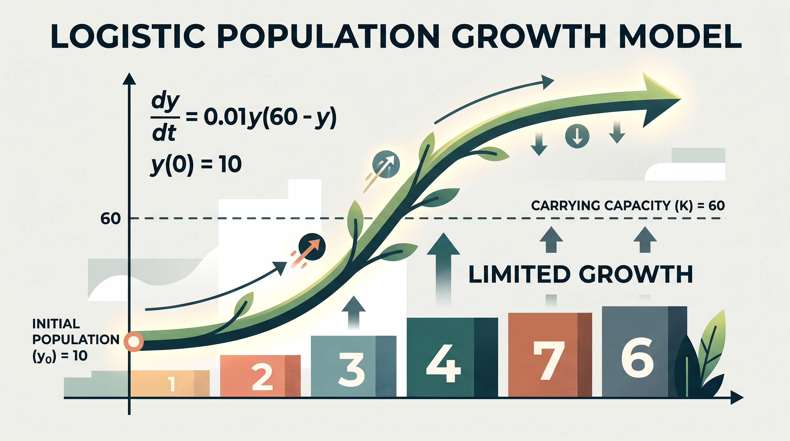
For $\frac{dy}{dt}=0.01y(60-y)$ with $y(0)=10$, determine whether the quantity initially increases or decreases and state its expected long-term behavior.
Since
$$ \frac{dy}{dt}
0.01(10)(60-10)>0, $$
the quantity initially increases. Because the initial value lies below the carrying capacity, the solution is expected to approach $y=60$ as $t\to\infty$, rather than grow without bound.
Source Materials
- Learn More (.pdf)
- AP Calculus AB and BC Course and Exam Description
- AP Calculus AB Course Overview
- AP Calculus Course at a Glance
- AP Calculus AB and BC Course at a Glance Poster
- Adopt AP Calculus AB
- AP Calculus AB
- AP Calculus AB
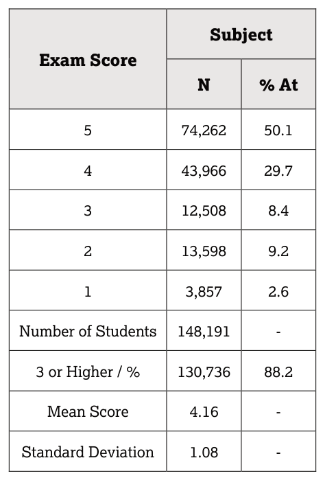
- Note: The number of students with Calculus AB subscores may differ slightly from the number of students who took the AP Calculus BC Exam due to exam administration incidents.