7.5 Approximating Solutions Using Euler’s Method (BC only)

7.5 Approximating Solutions Using Euler’s Method (BC only)

A differential equation can describe a changing system even when no convenient formula for the system exists. Euler’s method follows the local slope repeatedly: start at a known point, use the differential equation to estimate the slope there, and step forward to create an approximate solution curve.

BC-only scope: Topic 7.5, Approximating Solutions Using Euler’s Method, is BC-only. Topic 7.6, Finding General Solutions Using Separation of Variables, is part of the differential-equation progression for both AB and BC. Logistic growth models are also BC-only content.

The governing enduring understanding is FUN-7: “Solving differential equations allows us to determine functions and develop models.” The related learning objective is FUN-7.C: “Estimate solutions to differential equations.” The essential knowledge statement FUN-7.C.4 specifies that Euler’s method approximates either a solution to a differential equation or a point on a solution curve. The suggested skill is 1.E: Apply appropriate mathematical rules or procedures, with and without technology.

Euler’s method: turning slope into a path

Suppose a population satisfies

$$ \frac{dy}{dx}=f(x,y) $$

and the solution passes through the known point $(x_0,y_0)$. At that point, the differential equation gives the slope $f(x_0,y_0)$. For a step size $h$, Euler’s method estimates the next point by

$$ x_{n+1}=x_n+h, $$

$$ y_{n+1}=y_n+h f(x_n,y_n). $$

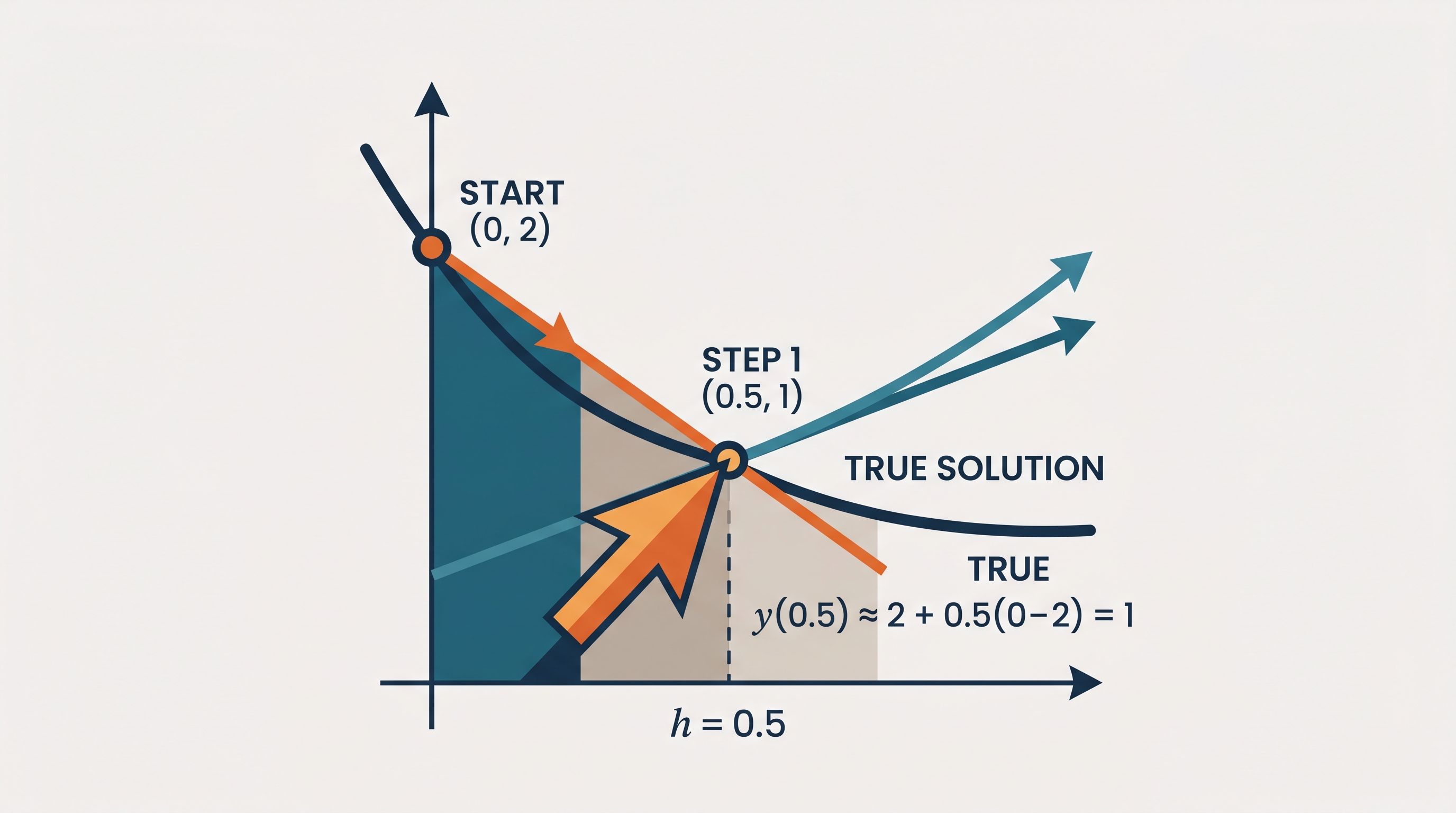
The essential idea is geometric: replace the unknown curve over a short interval by the tangent-line segment determined by the current point and current slope.

For example, approximate the solution to

$$ \frac{dy}{dx}=x+y $$

that passes through $(0,1)$ using step size $h=0.2$.

At $(x_0,y_0)=(0,1)$, the slope is

$$ f(0,1)=0+1=1. $$

Therefore,

$$ y_1=1+0.2(1)=1.2, \qquad x_1=0.2. $$

At $(0.2,1.2)$,

$$ f(0.2,1.2)=0.2+1.2=1.4, $$

so

$$ y_2=1.2+0.2(1.4)=1.48, \qquad x_2=0.4. $$

At $(0.4,1.48)$,

$$ f(0.4,1.48)=1.88, $$

and hence

$$ y_3=1.48+0.2(1.88)=1.856, \qquad x_3=0.6. $$

Thus the Euler estimate for $y(0.6)$ is approximately $1.856$.

The calculation uses the current point to determine the current slope. A frequent error is to use the new point $(x_{n+1},y_{n+1})$ inside $f(x,y)$ before that point has been computed. Another is to forget the factor $h$; the vertical change is not merely the slope, but

$$ \Delta y\approx h\cdot \text{slope}. $$

Graphing and judging an Euler approximation

A useful graphing procedure is:

1. Plot the initial point $(x_0,y_0)$.
2. Calculate the slope from the differential equation at that point.
3. Plot the next Euler point using the horizontal step $h$ and vertical change $h f(x_n,y_n)$.
4. Repeat the process for the required interval.
5. Connect consecutive points with short line segments, recognizing that the result is an approximation rather than the exact solution.
6. If technology supplies a direction field, compare the Euler segments with the small slope marks at each point.
7. Repeat with a smaller step size and compare the resulting paths.

A smaller step size usually produces a closer approximation because each line segment follows the changing slope for a shorter distance. However, “smaller” does not mean “exact”: Euler’s method still accumulates approximation error. If the curve bends strongly, a large step can jump noticeably away from the actual solution.

Euler’s method is often applied to population models. The logistic model below is a standard BC example: read its behavior from the equation first, then estimate values with Euler steps.

Logistic growth: limited resources create equilibria

A logistic model describes growth that slows as a population approaches a carrying capacity $K$:

$$ \frac{dP}{dt}=rP\left(1-\frac{P}{K}\right), $$

where $P$ is population, $r>0$ is the intrinsic growth constant, and $K>0$ is the carrying capacity.

The equilibrium solutions are

$$ P=0 \qquad\text{and}\qquad P=K. $$

If $0<P<K$, then $dP/dt>0$, so the population increases. If $P>K$, then $dP/dt<0$, so the population decreases toward $K$. The growth rate is greatest when $P=K/2$; near $0$ and near $K$, growth is slower.

For a BC-only Euler estimate, let

$$ \frac{dP}{dt}=0.4P\left(1-\frac{P}{1000}\right), \qquad P(0)=200, $$

with step size $h=1$. At $t=0$,

$$ P'(0)=0.4(200)\left(1-\frac{200}{1000}\right)=64. $$

Thus,

$$ P(1)\approx 200+1(64)=264. $$

At $P=264$,

$$ P'\approx 0.4(264)\left(1-\frac{264}{1000}\right)=77.7216, $$

so

$$ P(2)\approx264+77.7216=341.7216. $$

The population rises because it is below $K=1000$, but the model predicts eventual leveling rather than unlimited exponential growth.

For logistic equations, the equilibrium misconception is especially important: $K$ is not the initial population and does not mean the population instantly becomes $K$. It is the long-term balance level predicted by the model. A graph should show solutions below $K$ moving upward and solutions above $K$ moving downward.

Retrieval check

For

$$ \frac{dy}{dx}=x-y, \qquad y(0)=2, $$

with $h=0.5$, the first Euler estimate is

$$ y(0.5)\approx 2+0.5(0-2)=1. $$

Explain why the next slope must be evaluated at $(0.5,1)$, not at $(0,2)$, and identify the two equilibrium solutions of the logistic model