6.2 Approximating Areas with Riemann Sums

6.2 Approximating Areas with Riemann Sums

Topic 6.1 showed that accumulated change is the signed area under a rate graph. When the graph is curved, or the rate is known only at a few measured times, that area has no simple geometric formula. A Riemann sum approximates it with rectangles.

Suppose a storage tank’s rate of change, $R(t)$, is measured in liters per second, with time in seconds. The following values describe a piecewise-constant approximation based on the rate at the left endpoint of each interval.

Time interval (seconds)	Approximate rate (liters per second)	Signed accumulation (liters)
$0$ to $60$	$4$	$4(60)=240$
$60$ to $90$	$5$	$5(30)=150$
$90$ to $120$	$3$	$3(30)=90$
$120$ to $135$	$-1$	$-1(15)=-15$
$135$ to $150$	$-2$	$-2(15)=-30$

Each row of the table is one rectangle: a rate held constant across an interval, times the width of that interval. Adding the signed column gives a net change of about $435$ L.

Approximating curved accumulation with rectangles

A rate graph is often curved rather than piecewise constant. To approximate its accumulation, divide the interval into subintervals, choose a representative rate on each subinterval, and form rectangles:

$$ \text{approximate accumulation} \approx (\text{rate})(\text{interval width}) + (\text{rate})(\text{interval width}) +\cdots $$

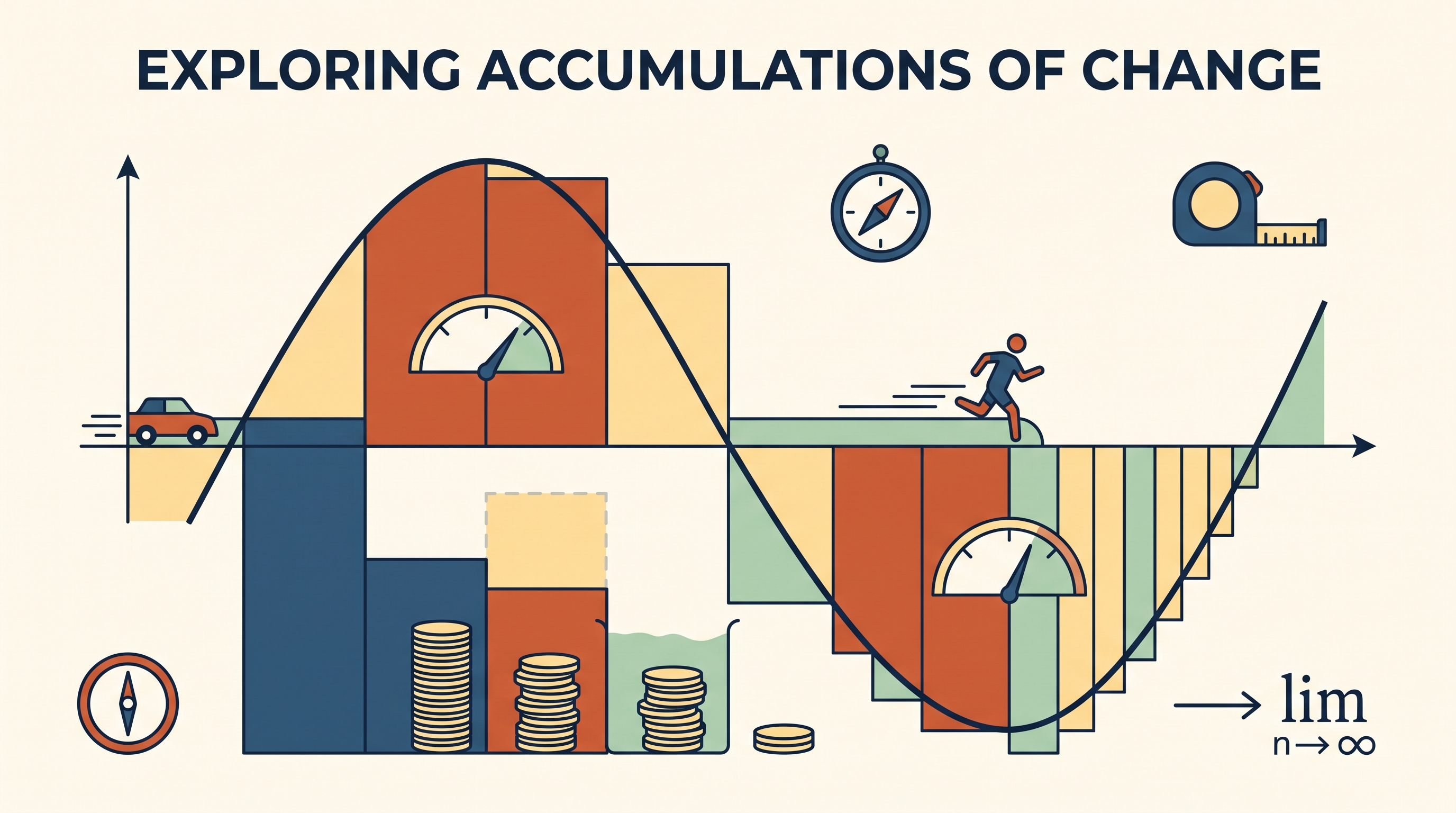
This procedure is a Riemann sum: a sum of rectangle areas used to approximate the area under a curve. Left-endpoint rectangles use the rate at the beginning of each subinterval; right-endpoint rectangles use the rate at the end. If the rate is increasing, left rectangles generally underestimate the positive accumulation, while right rectangles generally overestimate it.

The quality of an approximation depends on the rectangle widths and on how the function behaves. Narrower subintervals usually make the rectangles follow the curve more closely, but an approximation remains an approximation unless the exact accumulated value is determined by another method.

Applying the idea to data

For tabulated data at times $0$, $60$, $90$, $120$, $135$, and $150$ seconds, the interval widths are not all equal:

$$ 60,\quad 30,\quad 30,\quad 15,\quad 15. $$

Using one common width would misrepresent the accumulation. Each rate must be multiplied by the width of its own interval. In a real context, the result should be stated as a quantity and an interpretation—for example, “the tank gains approximately $435\text{ L}$ net,” rather than merely writing $435$.

Skill focus and retrieval check

Topic 6.2 emphasizes Skill 1.F: Explain how an approximated value relates to the actual value. Report the estimate with units, then say whether it is likely an overestimate or an underestimate, and why.

Retrieval check: A positive rate $r(t)$ is decreasing on $[0,6]$. With three equal subintervals, which is larger, the left or the right Riemann sum, and which one overestimates the accumulation? Answer: The left sum is larger and overestimates, because each left-endpoint height is the largest rate on its subinterval; the right sum underestimates.