7.4 Reasoning Using Slope Fields

7.4 Reasoning Using Slope Fields

Topic 7.3 built a slope field by drawing, at each point, a short segment with the slope the differential equation prescribes. This page uses the finished field. Without solving the equation, the segments show where solutions rise or fall, how quickly they change, and which constant solutions never move. The running example is $\frac{dy}{dx}=y-2$: its segments are horizontal along $y=2$, tilt upward above that line and downward below it.

A solution passing through a point must be tangent to the segments as it moves across the field.

Reasoning from a slope field

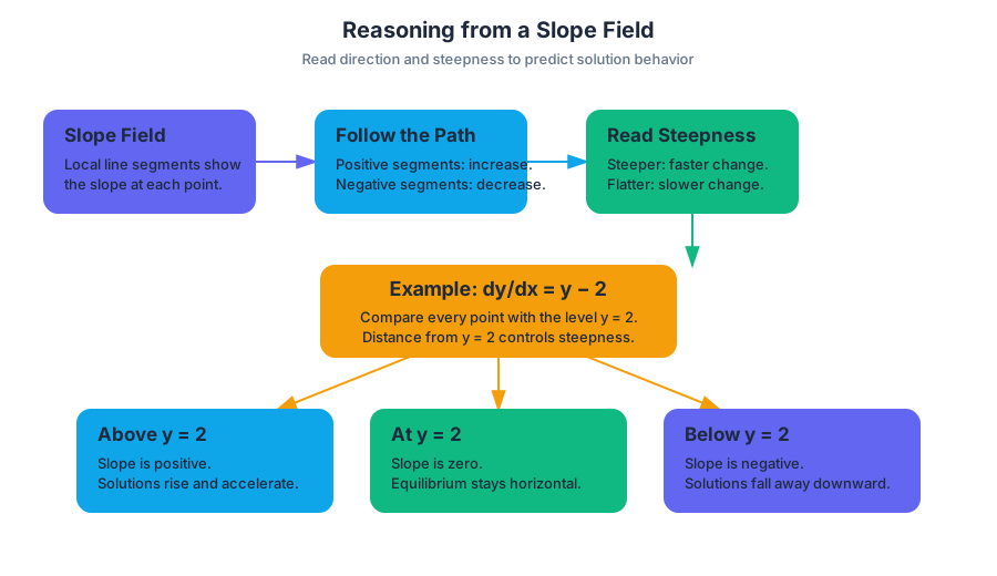
A slope field supports qualitative predictions even when no explicit formula for $y$ is available. If the segments along a solution’s path are positive, the solution increases; if they are negative, it decreases. Segments that become progressively steeper indicate faster change, while segments that flatten indicate slower change.

For $\frac{dy}{dx}=y-2$, a solution beginning at $(0,3)$ initially increases because its slope is $1$. As it rises above $y=2$, the slope becomes even larger, so the curve bends upward and moves away from $y=2$. A solution beginning at $(0,1)$ initially decreases because its slope is $-1$; below $y=2$, the field continues directing it downward.

The line $y=2$ is an equilibrium solution because its derivative is always zero there. A solution that starts exactly on this line remains horizontal.

Every solution follows the same field, so a slope field describes a whole family of solutions at once; an initial point selects one of them. To sketch the solution through a given point, start there and draw a smooth curve, in both directions, that stays tangent to the nearby segments. Follow the flow of the field rather than joining segments end to end. For $\frac{dy}{dx}=y-2$, a curve that starts above $y=2$ stays above it, and one that starts below stays below.

This work develops Mathematical Practice 2—Connecting Representations by moving between equations, slope fields, and verbal descriptions. It also uses Mathematical Practice 3—Justification when a conclusion is supported by slope signs or equilibrium lines, and Mathematical Practice 4—Communication and Notation when variables, derivatives, constants, and absolute values are written precisely.

Retrieval check

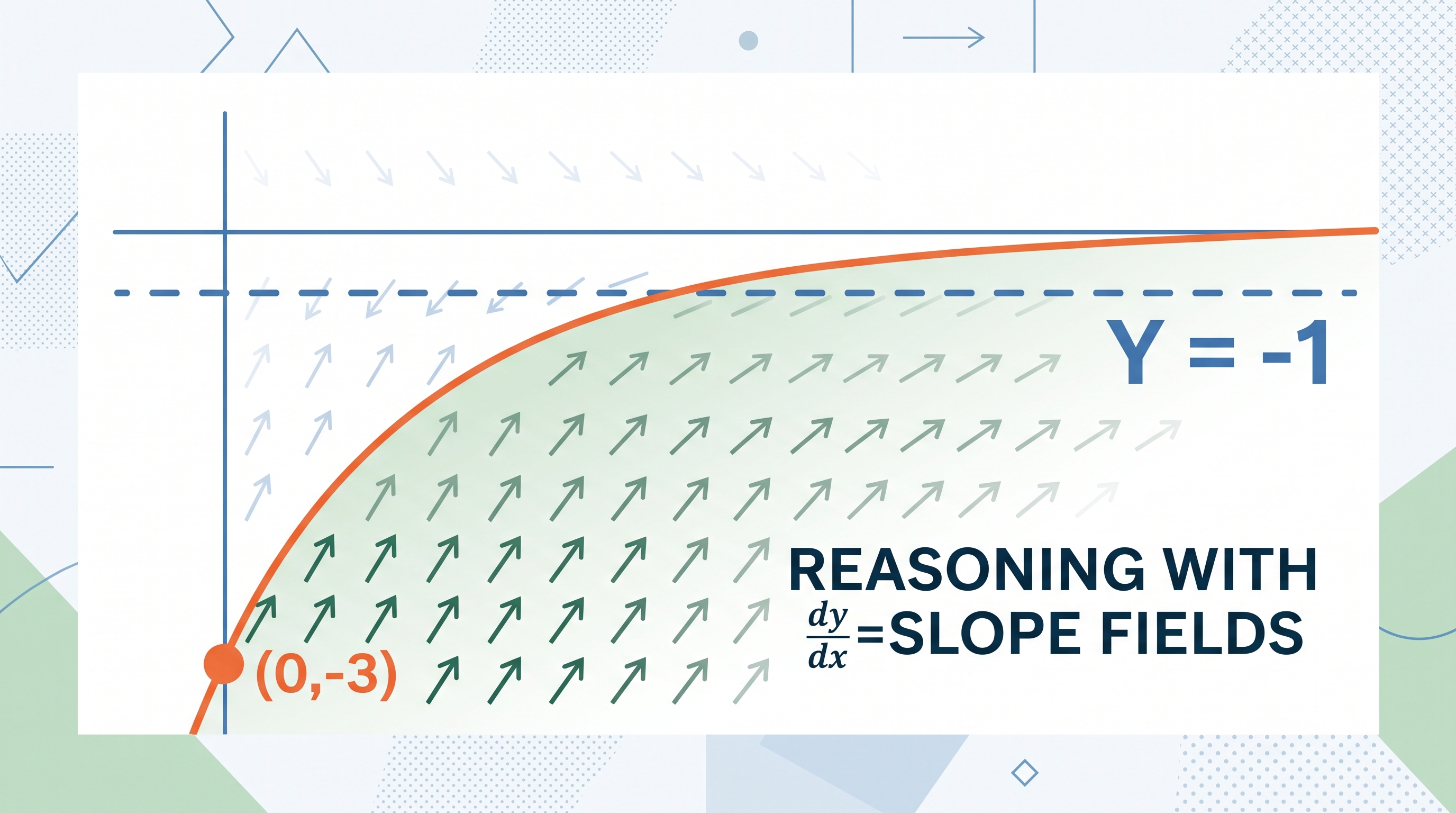
For the equation

$$\frac{dy}{dx}=-(y+1),$$

identify the horizontal line of equilibrium, state whether slopes are positive or negative above that line, and predict the direction of a solution beginning at $(0,-3)$.

The equilibrium line is $y=-1$. Below it, $y+1<0$, so $-(y+1)>0$ and the slopes are positive. Thus a solution beginning at $(0,-3)$ initially increases.