From the free course AP Calculus AB on Lykke
7.8 Exponential Models with Differential Equations
Key concepts: Solving differential equations to determine functions and develop models · Recognizing differential-equation forms that produce exponential models · Recognizing differential-equation forms that produce logistic models · Interpreting mathematical solutions in context · Exponential growth and decay models · Logistic models and carrying capacity
Why a rate proportional to the current amount gives the exponential model y = Ce^(kt), how to fit it to an initial value in context, and how it differs from logistic structure.
7.8 Exponential Models with Differential Equations
Topic 7.7 showed how separation of variables and an initial condition produce one particular solution. One differential equation appears so often in applications that its solution is worth recognizing on sight: when a quantity changes at a rate proportional to its current amount, the solution is always an exponential function. This page derives that model and applies it in context.
Enduring Understanding FUN-7: Solving differential equations allows us to determine functions and develop models.
Exponential models: recognize the form
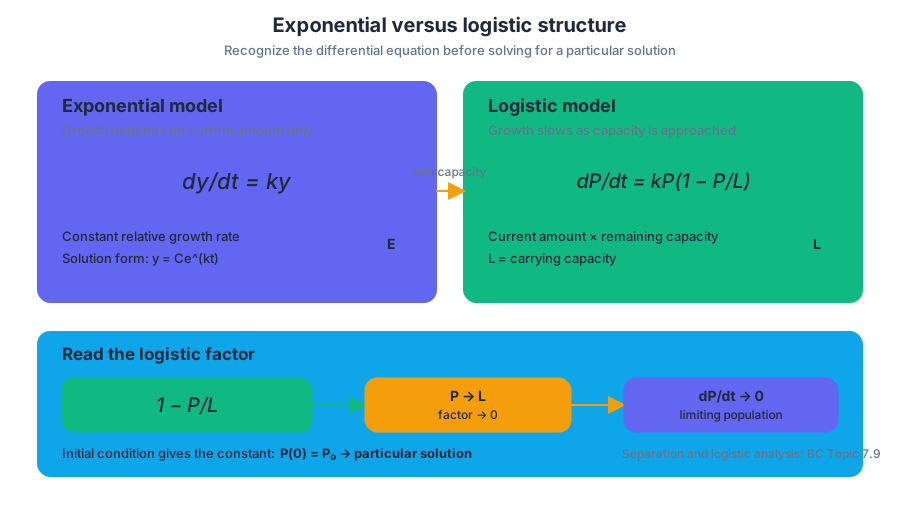
The differential equation $$ \boxed{\frac{dy}{dt}=ky} $$ produces an exponential model because the rate of change is proportional to the current amount. Separating and integrating gives $$ \frac{1}{y},dy=k,dt \quad\Longrightarrow\quad \ln|y|=kt+C, $$ which rearranges to $$ y=Ce^{kt}. $$
If $k>0$, the model describes exponential growth; if $k<0$, it describes exponential decay. The constant $C$ is determined by an initial value. In context, $k$ has units of inverse time, while $y$ has the units of the modeled quantity.
Contextual example: population growth
A laboratory culture begins with $50$ organisms and grows at a rate proportional to its current population: $$ \frac{dP}{dt}=0.2P, \qquad P(0)=50. $$ The general solution is $P=Ce^{0.2t}$. Applying $P(0)=50$ gives $50=C$, so $$ \boxed{P(t)=50e^{0.2t}}. $$ After $5$ time units, $$ P(5)=50e^1\approx 135.914. $$ The model predicts approximately $136$ organisms, subject to the assumptions of continuous proportional growth.
Exponential versus logistic structure
A logistic differential equation includes a capacity-limiting factor: $$ \boxed{\frac{dP}{dt}=kP\left(1-\frac{P}{L}\right)}. $$ Here, $P$ is the current amount and $L$ is the carrying capacity. The product $P\left(1-\frac{P}{L}\right)$ distinguishes logistic growth from $\frac{dy}{dt}=ky$: growth depends both on the current amount and on the remaining capacity.
When $P$ approaches $L$, the factor $1-\frac{P}{L}$ approaches $0$, so the rate approaches $0$. Thus $L$ is the limiting population value, or carrying capacity. Recognizing this form is required for identifying logistic models; solving and analyzing logistic equations belong to the BC-only treatment of Topic 7.9.
Applications and representations
Differential-equation models can describe motion along a line as well as population change. If $s(t)$ is position, then $s'(t)=v(t)$ is velocity; a rule such as $\frac{dv}{dt}=kv$ models how velocity changes, while the initial position or velocity selects a particular motion. A strong solution connects the verbal situation, differential equation, graph or slope field, and final function.
This work develops 1.E — Apply appropriate mathematical rules or procedures, with and without technology: separation, antidifferentiation, logarithm rules, constant selection, and algebraic rearrangement must remain visible. It also exercises the representation and modeling processes associated with [2.C], [3.G], and [4.D] by translating among equations, conditions, graphs, context, and notation.
Retrieval check: A radioactive sample decays at a rate proportional to the amount present, with $k=-0.1$ per year and $A(0)=80$ grams. Write the model and find $A(10)$. The equation $\frac{dA}{dt}=-0.1A$ has exponential form, so $A(t)=80e^{-0.1t}$ and $A(10)=80e^{-1}\approx 29.4$ grams.
Source Materials
- Learn More (.pdf)
- AP Calculus AB and BC Course and Exam Description
- AP Calculus AB Course Overview
- AP Calculus Course at a Glance
- AP Calculus AB and BC Course at a Glance Poster
- Adopt AP Calculus AB
- AP Calculus AB
- AP Calculus AB
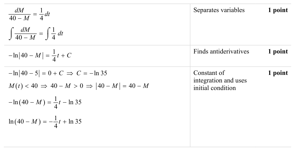
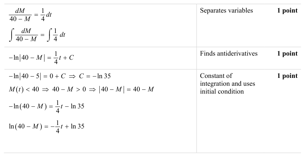
- equation ( ) 1 40 4 dM M dt = − with initial condition ( ) 0 5. M =
- equation ( ) 1 40 4 dM M dt = − with initial condition ( ) 0 5. M =