From the free course AP Calculus AB on Lykke
6.5 Interpreting the Behavior of Accumulation Functions Involving Area
Key concepts: Accumulation functions defined by definite integrals · Interpreting accumulation functions involving area · Accumulation of change · Using definite integrals to define new functions · Differentiating accumulation functions · Relating mathematical characteristics across representations
How to read where an accumulation function rises, falls, bends and has extrema from the graph of its rate, using signed area for its values.
6.5 Interpreting the Behavior of Accumulation Functions Involving Area
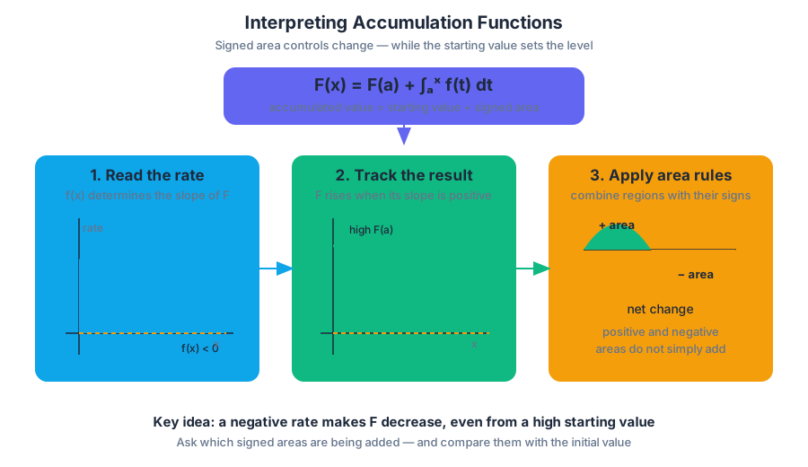
An accumulation graph can stay high even while its associated rate is negative: it is falling, but from the larger value that earlier positive accumulation built up. The key question is not merely “How much area is present?” but which signed areas are being added, and how do they change the function’s behavior?
Reading an accumulation function through its rate
Suppose $G(x)$ records the net amount accumulated from a starting location to $x$, while $f(x)$ is the rate being accumulated. The load-bearing relationship from the preceding topic is
$$G'(x)=f(x).$$
This single connection lets us translate between representations:
| Information about $f$ | Consequence for $G$ |
|---|---|
| $f(x)>0$ | $G$ is increasing |
| $f(x)<0$ | $G$ is decreasing |
| $f(x)=0$ | $G$ has a horizontal tangent, possibly a local extremum |
| $f$ is increasing | $G$ is concave up |
| $f$ is decreasing | $G$ is concave down |
The word net matters. Area above the $x$-axis contributes positively, while area below the $x$-axis contributes negatively. Thus, a definite integral can represent both accumulated change and signed area—not always ordinary geometric area.
Worked interpretation: area controls the graph
Let
$$G(x)=\int_0^x f(t),dt,$$
where the graph of $f$ is below the $x$-axis on $0<x<3$, crosses the axis at $x=3$, and is above the axis on $3<x<6$. Without calculating an antiderivative, interpret $G$.
Because $f(x)<0$ on $(0,3)$, $G$ decreases there. At $x=3$, the accumulation graph has a horizontal tangent because $f(3)=0$. Since $f(x)>0$ on $(3,6)$, $G$ increases there. Therefore, $G$ has a local minimum at $x=3$, provided the sign changes from negative to positive.
If the region below the axis from $0$ to $3$ has area $8$ and the region above the axis from $3$ to $5$ has area $11$, then
$$G(3)=-8$$
and
$$G(5)=-8+11=3.$$
The function does not “forget” the first region: the later positive area first cancels the earlier deficit and then creates a positive net accumulation.
When the upper limit is a function of $x$
When an accumulation expression contains a variable limit, differentiate it to reveal the matching rate. For example, if
$$H(x)=\int_2^{x^3}\sqrt{1+t^2},dt,$$
then the variable endpoint contributes a chain-rule factor:
$$H'(x)=\sqrt{1+(x^3)^2}\cdot 3x^2 =3x^2\sqrt{1+x^6}.$$
The common error is to write only $\sqrt{1+x^6}$ and forget that the upper limit is $x^3$, not $x$. This is the missing chain-factor misconception: a variable boundary changes at its own rate.
Skill focus and retrieval check
These tasks explicitly develop 2.D Identify how mathematical characteristics or properties of functions are related in different representations, especially when a graph of $f$, an accumulation graph $G$, and an integral communicate the same behavior. They also develop 3.D Apply an appropriate mathematical definition, theorem, or test when using signed area, integral properties, and derivative-based behavior.
Retrieval check: If $f$ is negative and decreasing on an interval, what must be true about $G$ there, where $G'(x)=f(x)$? Answer: $G$ is decreasing and concave down. If $\int_0^4 f(x),dx=6$ and $\int_4^7 f(x),dx=-9$, then $\int_7^0 f(x),dx=3$.
Source Materials
- Learn More (.pdf)
- AP Calculus AB and BC Course and Exam Description
- AP Calculus AB Course Overview
- AP Calculus Course at a Glance
- AP Calculus AB and BC Course at a Glance Poster
- Adopt AP Calculus AB
- AP Calculus AB
- AP Calculus AB
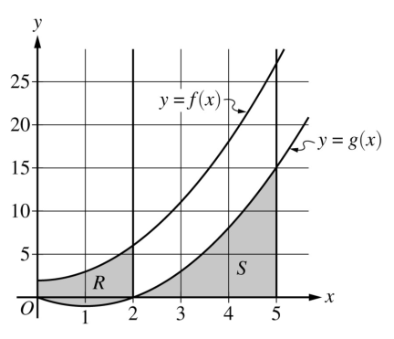
- T he functions f and g are defined by f (x) = x2 + 2 and g(x) = x2 - 2x, as shown in the graph.
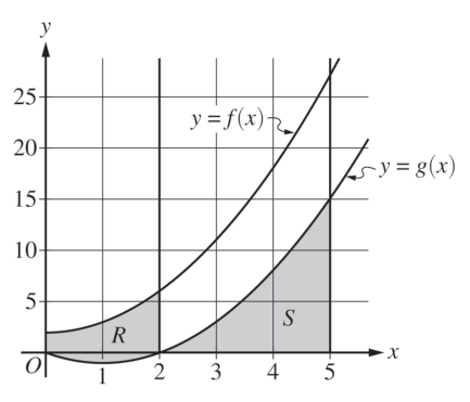
- 6. The functions f and g are defined by f x x 2 2 = + ( ) and g x x x 2 2 = ( ) − , as shown in the graph.