1.3 The Power of Geographic Data

1.3 The Power of Geographic Data

A map becomes geographically powerful when it does more than show where something is: it helps explain why that pattern occurs, how places are connected, and what changes across scale. A set of numbers can show that one neighborhood has more restaurants than another; combining those numbers with location, transportation, income, and land-use information can suggest why the restaurants cluster there.

Geographic data become analytically powerful when quantitative evidence is connected to spatial relationships, geographic context, and processes operating across places.

From data to geographic explanation

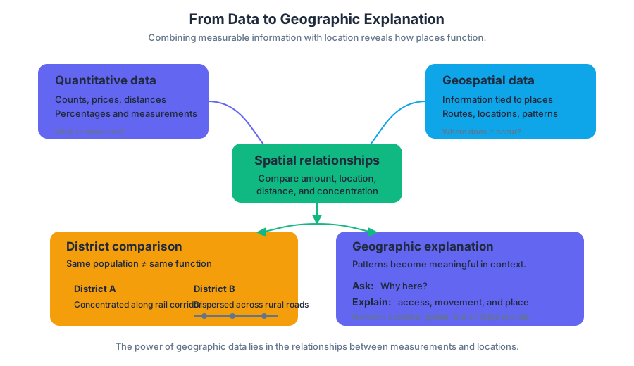
The previous topic established that geographic information can come from field observations, surveys, censuses, GPS, remote sensing, GIS, and other sources. Organizations and individuals may also gather information directly in the field. Here, the key step is not collecting another type of data; it is combining quantitative data—measurable information such as population counts, prices, distances, or percentages—with geospatial data, information linked to specific locations on Earth.

Geographers use quantitative and spatial relationships to analyze complex issues. A table might report that two districts have similar populations, while a map reveals that one district is concentrated along a rail corridor and the other is dispersed across rural roads. The numerical similarity does not mean the places function in the same way.

Worked example: explaining a restaurant pattern

Suppose a city records the locations of $120$ new restaurants, average household income, pedestrian counts, and distances to rail stations.

1. Quantitative evidence: The highest pedestrian counts occur near rail stations, and restaurant openings are more common in higher-income districts.
2. Geospatial evidence: The restaurants form visible clusters along transit lines rather than spreading evenly across the city.
3. Spatial relationship: The cluster connects restaurants with accessibility and concentrated foot traffic.
4. Geographic explanation: Restaurant growth is likely shaped by the interaction of consumer purchasing power, transportation access, and the movement of people through particular places.

The conclusion is stronger than “restaurants are more numerous in District A.” It identifies a relationship among economic, cultural, and spatial factors. It also remains appropriately cautious: the data show association, but they do not automatically prove that income alone caused the pattern.

Geographic perspectives

A geographic perspective is a way of interpreting an issue by asking how location, scale, connections among places, and human–environment relationships shape it. The same restaurant pattern can produce different explanations depending on the perspective used.

Geographic perspective	Guiding question in the restaurant example
Spatial	Where are restaurants clustered, and what relationships connect them to transit, roads, or customers?
Regional	Does the pattern distinguish one part of the city from another, creating a recognizable region?
Human–environment	How do terrain, available land, environmental conditions, or infrastructure affect where restaurants can operate?

These perspectives work together rather than compete. A spatial analysis may identify a cluster; a regional analysis may show that the cluster belongs to a rapidly redeveloping corridor; a human–environment analysis may reveal that a river, steep slope, or floodplain limits expansion.

Scale changes the pattern

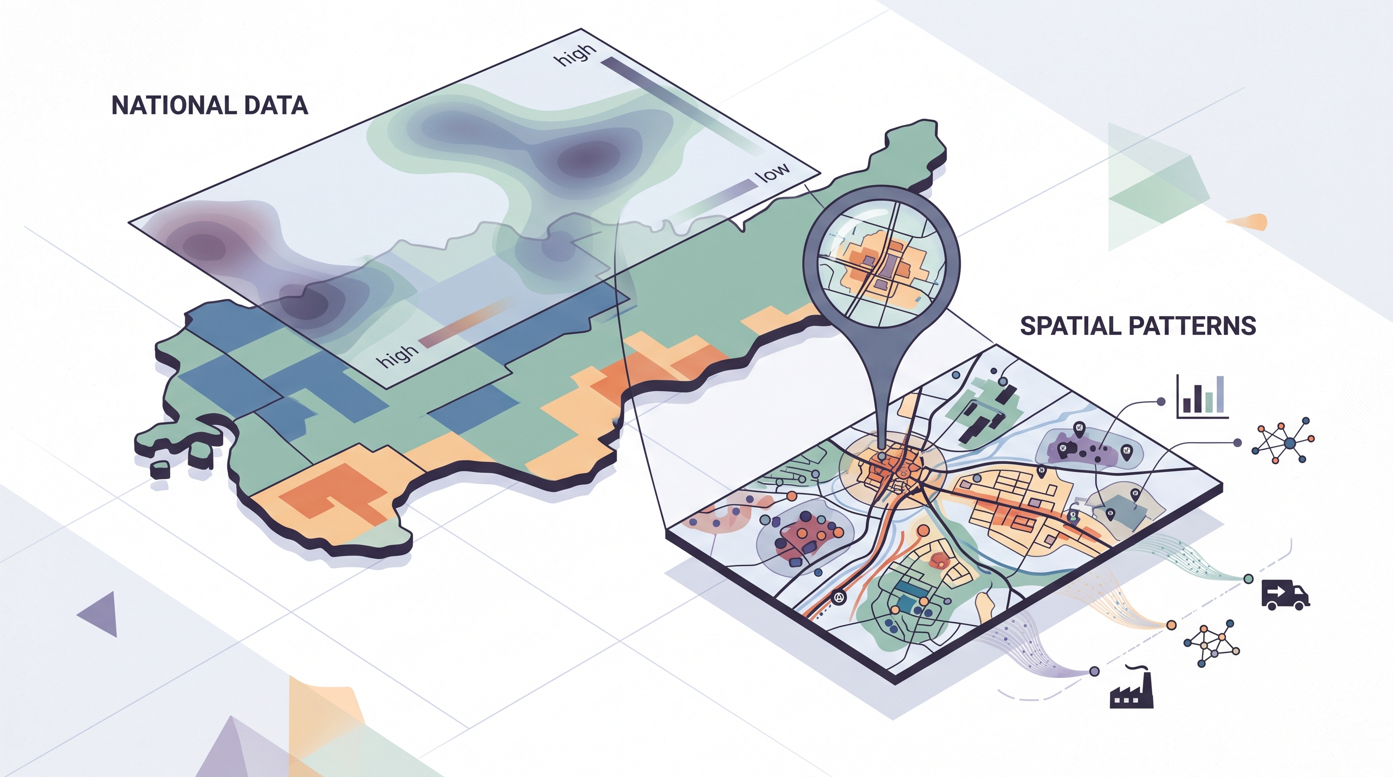
Scale of analysis is the geographic level at which data are examined. It may be global, regional, national, or local. The pattern visible at one scale may weaken, disappear, or reverse at another.

Consider air pollution. At the global scale, emissions may appear concentrated in major industrial economies. At the national scale, the pattern may vary by energy policy and industrial geography. At the local scale, pollution may be highest beside a highway or factory, even within a generally low-pollution region.

This principle is captured by PSO-1.C.1, which identifies global, regional, national, and local scales of analysis, and PSO-1.D.1, which emphasizes that patterns and processes at different scales can produce variations in, and different interpretations of, data. Maps and data must therefore be interpreted in relation to the context and scale in which they are presented.

Patterns, processes, and changing connections

A spatial pattern is the arrangement of features across space; a process is an action or change that produces, maintains, or transforms that arrangement. Geographers analyze relationships among and between places to reveal important patterns and processes, including environmental, economic, cultural, and political relationships.

Modern transportation and communication can make distant places interact more quickly and frequently. This broad condition is associated with time-space compression and time-space convergence: technological change reduces the practical effects of distance by accelerating connections. The important analytical question is not simply whether places are connected, but which places gain access, at what scale, and with what consequences.

Examiner’s misconception check — “The map proves the cause.”
A visible cluster shows a pattern, not automatically its cause. A strong geographic explanation identifies evidence, names a spatial relationship or process, and connects that relationship to the geographic context and scale.

Skill focus: Data Analysis 3.B — Describe spatial patterns presented in maps and in quantitative and geospatial data

For Data Analysis 3.B, move from observation to interpretation: describe the pattern accurately, identify relevant relationships, and explain what the pattern may reveal. Also apply Scale Analysis 5.A — Identify the scales of analysis presented by maps, quantitative and geospatial data, images, and landscapes when deciding whether a conclusion applies locally, regionally, nationally, or globally.

Retrieval check: A map shows similar unemployment rates for two countries, but one country’s unemployment is concentrated in a few industrial regions while the other’s is widespread. What did the national scale conceal, and what additional scale or geospatial evidence would help explain the difference? Include the pattern, the scale, and one possible process.