8.3 Population Ecology

8.3 Population Ecology

A population can double rapidly, stall at a limit, or collapse when births, deaths, immigration, and emigration change the balance of individuals. Population ecology examines these changes quantitatively: not simply how many organisms exist, but how population size, density, distribution, and growth change through time.

Investigative question: What determines whether a population grows exponentially, levels off, or declines?

CED alignment: Topic 8.3 Population Ecology; Learning Objective 8.3.A; Essential Knowledge 8.3.A.1, 8.3.A.2, 8.3.A.3, and 8.3.A.4. The topic is assessed especially through Science Practice 2: Visual Representations, Science Practice 4: Representing and Describing Data, Science Practice 5: Statistical Tests and Data Analysis, and Science Practice 6: Argumentation.

Population size is a balance, not a single rate

Population size is the number of individuals in a population. Its change depends on four demographic processes:

$$\Delta N = (B + I) - (D + E)$$

where $N$ is population size, $B$ is births, $I$ is immigration, $D$ is deaths, and $E$ is emigration. Births and immigration add individuals; deaths and emigration remove them.

Two populations may contain the same number of organisms but have very different ecological conditions. Population density is the number of individuals per unit of area or volume:

$$\text{Population density}=\frac{\text{number of individuals}}{\text{area or volume}}$$

A population of $200$ plants spread across $100\ \text{m}^2$ has a density of $2\ \text{plants}\cdot\text{m}^{-2}$. If the same $200$ plants occupy $20\ \text{m}^2$, density is $10\ \text{plants}\cdot\text{m}^{-2}$.

Population dispersion describes how individuals are arranged in space. A clumped pattern may occur when resources are patchy or when organisms live socially. Uniform spacing can result from territorial behavior or competition. Random spacing occurs when individuals neither strongly attract nor repel one another. Dispersion is different from density: density asks how many; dispersion asks how arranged.

Exponential growth: the J-shaped model

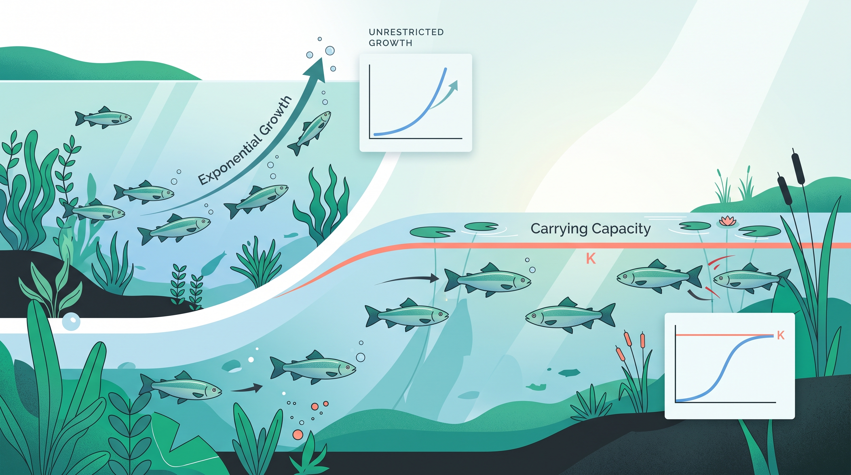
When resources are effectively unlimited, a population can grow at a rate proportional to its current size. This is exponential growth, represented by a J-shaped curve:

$$\frac{dN}{dt}=rN$$

Here, $r$ is the per-capita rate of increase and $N$ is population size. The larger the population becomes, the more individuals are available to reproduce, so the absolute increase becomes faster.

Worked example: Suppose a bacterial population begins with $100$ cells and doubles every hour. After one hour it has $200$ cells; after two hours, $400$; after three hours, $800. The increase is not a constant number of cells per hour—the population adds $100$, then $200$, then $400$. That accelerating pattern is the signature of exponential growth.

Exponential growth is most plausible for a population entering a new environment with abundant resources, few predators, and little competition. It cannot continue indefinitely because every real environment imposes limits.

Logistic growth: the S-shaped model

Logistic growth incorporates environmental limits. The population initially grows almost exponentially, but growth slows as the population approaches the environment’s carrying capacity, $K$—the largest population size that the environment can sustain over time.

$$\frac{dN}{dt}=rN\left(\frac{K-N}{K}\right)$$

When $N$ is far below $K$, the factor $\frac{K-N}{K}$ is relatively large and growth is rapid. As $N$ approaches $K$, that factor approaches zero, so net growth slows and the curve levels into an S shape.

At carrying capacity, individuals are still being born and dying. Carrying capacity does not mean that reproduction stops; it means that, on average, births plus immigration balance deaths plus emigration. Because environmental conditions fluctuate, $K$ is usually a dynamic estimate rather than a permanent, perfectly fixed number.

Misconception check: “A population at $K$ never changes”

This is the carrying-capacity equilibrium misconception. A population near $K$ may rise above it, fall below it, or fluctuate around it. Drought, disease, seasonal food availability, and changes in predation can all shift the population and may also change the value of $K$ itself.

A second common error is treating $r$ as the number of new individuals. It is a per-capita rate: the average contribution of each individual to population increase. A population with a modest $r$ can still add many organisms if $N$ is large.

AP reasoning in population models

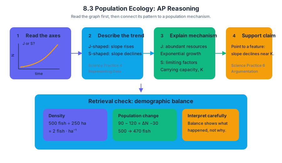
For a graph, first identify the axes and determine whether the curve is J-shaped or S-shaped. Then connect the pattern to mechanism: accelerating growth suggests abundant resources and exponential growth; leveling suggests limiting factors and carrying capacity. Under Science Practice 4: Representing and Describing Data, describe the trend before explaining it. Under Science Practice 6: Argumentation, support the explanation with a specific feature of the graph, such as a declining slope near $K$.

Retrieval check: A fish population contains $500$ individuals in a lake covering $250\ \text{ha}$. Its density is $2\ \text{fish}\cdot\text{ha}^{-1}$. If births and immigration total $90$ fish while deaths and emigration total $120$, then $\Delta N=-30$: the population declines to $470$ fish, assuming no other changes. Is that decline caused by density alone? No—the demographic balance shows what happened; identifying the environmental cause requires additional evidence.