7.5 Hardy–Weinberg Equilibrium

7.5 Hardy–Weinberg Equilibrium

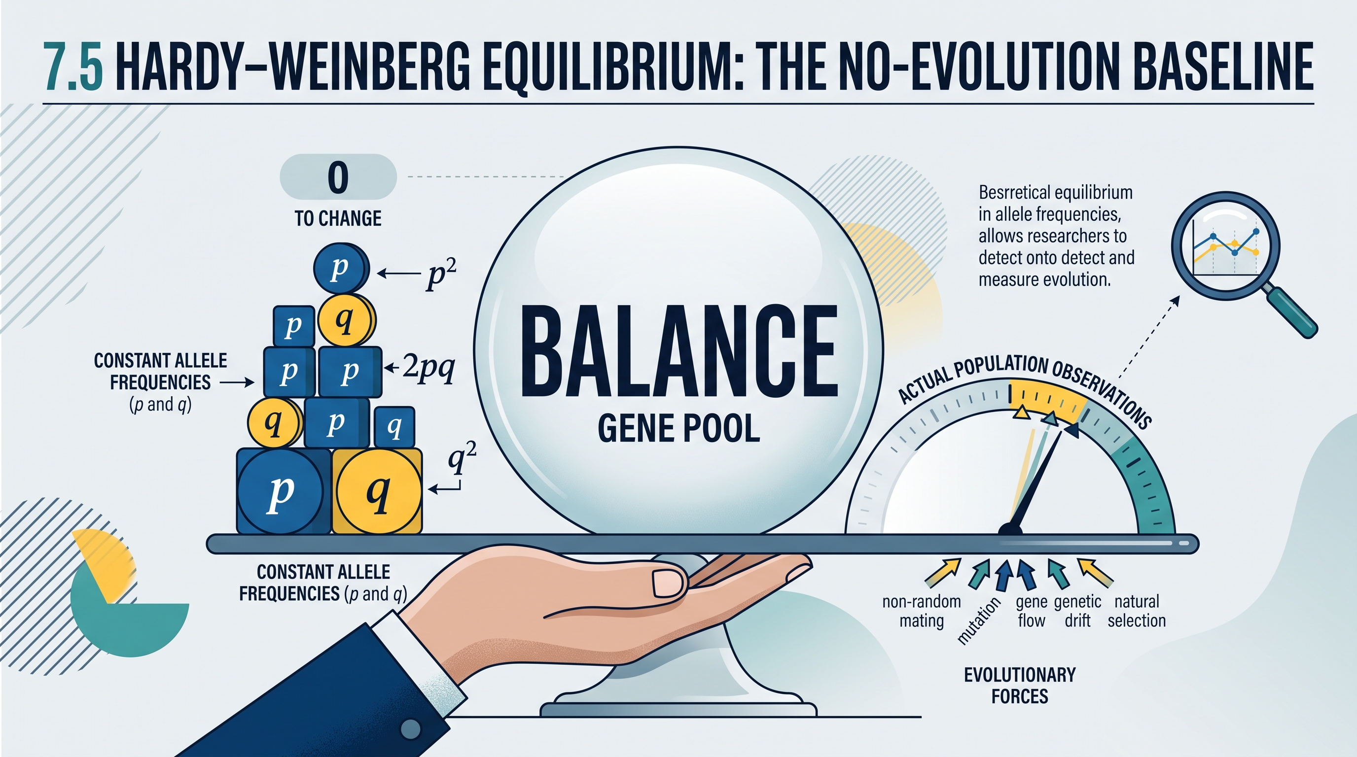
A population can evolve without any individual organism changing its genes: evolution is detected when allele frequencies—the proportions of different alleles in a population—change across generations. The Hardy–Weinberg model provides the mathematical “still photograph” against which that change can be measured.

Hardy–Weinberg equilibrium is the predicted genetic state of a population in which allele and genotype frequencies remain constant from generation to generation.

The model: from alleles to genotypes

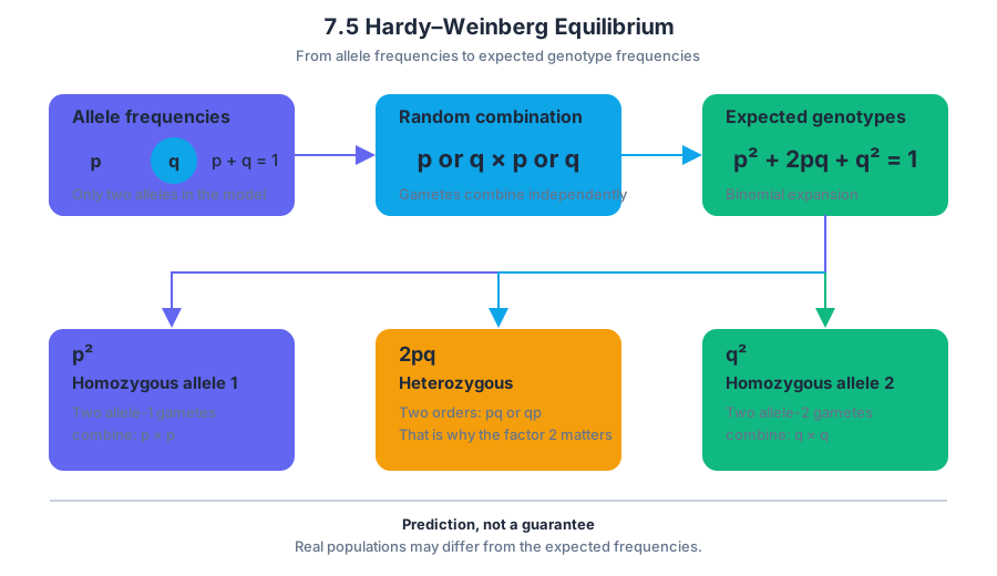
Imagine a gene with two alleles. Let $p$ represent the frequency of allele $1$ and $q$ represent the frequency of allele $2$. Because these are the only two alleles in the model, their frequencies must sum to the whole population:

$$p+q=1$$

If gametes combine randomly, the expected genotype frequencies follow the binomial expansion:

$$p^2+2pq+q^2=1$$

The terms have precise meanings:

Mathematical term	Genotype represented	Meaning
$p^2$	Homozygous for allele $1$	Two allele-$1$ gametes combine
$2pq$	Heterozygous	Either allele-$1$ then allele-$2$, or allele-$2$ then allele-$1$
$q^2$	Homozygous for allele $2$	Two allele-$2$ gametes combine

The factor $2$ in $2pq$ matters because the two alleles can occur in either order: $pq$ or $qp$. The equation predicts genotype frequencies from allele frequencies; it does not claim that every real population will match the prediction perfectly.

Worked example: calculating the expected population

Suppose allele $1$ has frequency $p=0.70$ in a population. First calculate the other allele:

$$q=1-p=1-0.70=0.30$$

The expected genotype frequencies are then:

$$p^2=(0.70)^2=0.49$$

$$2pq=2(0.70)(0.30)=0.42$$

$$q^2=(0.30)^2=0.09$$

Thus, the model predicts $49%$ homozygous allele-$1$, $42%$ heterozygous, and $9%$ homozygous allele-$2$. These add to $1.00$, or $100%$. If the population contains $1{,}000$ individuals, the expected genotype counts are $490$, $420$, and $90$, respectively.

Equilibrium as a null hypothesis

The Hardy–Weinberg model is a null hypothesis: it predicts what would happen if no evolutionary process altered allele frequencies. A population or allele in Hardy–Weinberg equilibrium is therefore not evolving with respect to that gene under the model.

The required conditions are idealized:

• a very large population;
• random mating;
• no mutation;
• no migration, or gene flow;
• no natural selection favoring one allele or genotype;
• no other process systematically changing allele frequencies.

These conditions are never fully met in nature. Their value is practical: if observed genotype frequencies differ substantially from Hardy–Weinberg predictions, the difference suggests that one or more evolutionary processes may be operating. The model gives scientists a baseline rather than a claim that real populations are perfectly static.

Why population size matters

In a small population, genetic drift—random change in allele frequencies caused by chance sampling—can overwhelm other evolutionary effects. Imagine a classroom population in which only a few individuals reproduce. By chance alone, one allele may become common or disappear, even if neither allele improves survival.

This is why a small laboratory simulation can be misleading: its population may be too small to approximate the large-population condition. A mathematical model or spreadsheet can instead represent a theoretically very large population and reveal the expected inheritance pattern without drift dominating the result.

Connecting the model to evolution

Hardy–Weinberg analysis becomes powerful when repeated generations are compared. If allele frequency changes from $p=0.70$ to $p=0.62$, then the population is evolving for that gene, regardless of whether the cause is mutation, genetic drift, gene flow, a bottleneck, or natural selection.

A strong scientific argument follows this chain:

$$ \text{calculate allele frequencies} \rightarrow \text{predict } p^2,\ 2pq,\ q^2 \rightarrow \text{compare with observations} \rightarrow \text{identify possible evolutionary change} $$

For example, a bottleneck can randomly remove individuals and alter allele frequencies; gene flow can introduce alleles from another population; mutation can create a new allele; and drift can shift frequencies especially strongly in small populations. The model helps distinguish “genotypes differ from expectation” from the stronger conclusion “allele frequencies changed over time.”

Misconception check

Misconception: Hardy–Weinberg equilibrium describes what evolution does.
Correction: It describes what allele frequencies would do in the absence of evolutionary change. It is the standard used to detect evolution, not a force that prevents evolution.

CED alignment: This topic develops Learning Objective 7.5.A and Essential Knowledge 7.5.A.1, applying mathematical models to allele and genotype frequencies. The principal science practices are Science Practice 2: Visual Representations, when translating between equations and population models; Science Practice 4: Representing and Describing Data, when organizing observed and expected frequencies; Science Practice 5: Statistical Tests and Data Analysis, when evaluating deviations; and Science Practice 6: Argumentation, when using calculations and experimental data to argue whether a population is evolving.

Retrieval check: A population has $q=0.20$. What are $p$, $p^2$, $2pq$, and $q^2$? If the allele frequencies are different in the next generation, is the population in Hardy–Weinberg equilibrium? Explain why in one sentence.