5.3 Concentration Changes Over Time · 5.4 Elementary Reactions

5.3 Concentration Changes Over Time · 5.4 Elementary Reactions

A reaction’s changing concentration is a chemical clock: the shape of the data reveals the reaction order, the slope reveals the rate constant, and the mechanism explains which molecular event controls the observed rate.

From concentration data to reaction order

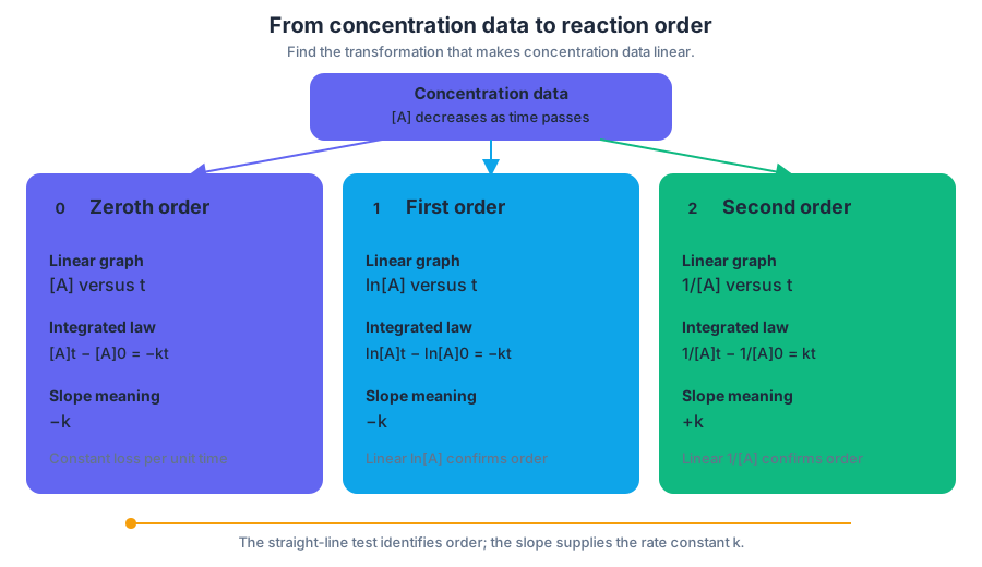
For a reactant $A$, concentration-versus-time data show how quickly $[A]$ decreases. The decisive test is not merely whether the graph slopes downward, but which transformation of concentration produces a straight line.

Reaction order in $A$	Linear graph	Integrated rate law	Meaning of slope
Zeroth order	$[A]$ versus $t$	$[A]_t-[A]_0=-kt$	$-k$
First order	$\ln[A]$ versus $t$	$\ln[A]_t-\ln[A]_0=-kt$	$-k$
Second order	$1/[A]$ versus $t$	$\frac{1}{[A]_t}-\frac{1}{[A]_0}=kt$	$+k$

These relationships preserve the essential knowledge statements 5.3.A.1, 5.3.A.2, 5.3.A.3, and 5.3.A.4: reaction order can be inferred from concentration data; a first-order reaction gives a linear $\ln[A]$-versus-time plot; a second-order reaction gives a linear $1/[A]$-versus-time plot; and the slope supplies the rate constant.

Worked example: identifying order and $k$

Suppose a reactant has the following measured concentrations:

$t$ in $s$	$[A]$ in $M$	$\ln[A]$	$1/[A]$ in $M^{-1}$
$0$	$0.100$	$-2.303$	$10.0$
$20$	$0.0500$	$-2.996$	$20.0$
$40$	$0.0250$	$-3.689$	$40.0$

The concentration halves every $20\ \mathrm{s}$. More decisively, $\ln[A]$ decreases by approximately $0.693$ during each equal time interval, so $\ln[A]$ versus $t$ is linear. The reaction is first order, and

$$ k=-\text{slope} =-\frac{-2.996-(-2.303)}{20\ \mathrm{s}} =3.47\times10^{-2}\ \mathrm{s^{-1}}. $$

The first-order integrated law predicts the concentration at $t=60\ \mathrm{s}$:

$$ \ln[A]_{60}-\ln(0.100) =-(3.47\times10^{-2})(60), $$

$$ [A]_{60}=0.0125\ \mathrm{M}. $$

Misconception check — “The steepest concentration graph identifies the order.” It does not. A graph of $[A]$ versus $t$ can curve for a first- or second-order reaction, and its visual steepness depends on the starting concentration and units. Test $[A]$, $\ln[A]$, and $1/[A]$ systematically.

Half-life and units of $k$

A half-life, $t_{1/2}$, is the time required for a reactant concentration to fall to one-half its current value. For a first-order reaction, the half-life is constant:

$$ t_{1/2}=\frac{\ln 2}{k}. $$

For the worked example,

$$ t_{1/2}=\frac{0.693}{3.47\times10^{-2}\ \mathrm{s^{-1}}} =20.0\ \mathrm{s}. $$

This constancy is diagnostic: equal concentration-halving intervals support first-order behavior. The units of $k$ depend on overall reaction order: $\mathrm{s^{-1}}$ for first order, $\mathrm{M,s^{-1}}$ for zeroth order, and $\mathrm{M^{-1},s^{-1}}$ for second order. Misconception check — “$k$ always has units of $\mathrm{s^{-1}}$.” Only a first-order rate constant does.

Beer’s law: turning color into concentration

Spectrophotometry measures how strongly a solution absorbs light. Beer’s law connects absorbance, $A_{\mathrm{abs}}$, to concentration:

$$ A_{\mathrm{abs}}=\varepsilon bc, $$

where $\varepsilon$ is the molar absorptivity, $b$ is the path length of the cuvette, and $c$ is concentration. If $\varepsilon$ and $b$ remain constant, absorbance is directly proportional to concentration.

In the fading crystal violet investigation, the purple reactant becomes less concentrated as the reaction proceeds, so its absorbance decreases. A calibration relationship—or a constant proportionality when conditions permit—converts each absorbance measurement into $[\mathrm{CV}^+]$. The resulting concentration data can then be tested using $[A]$, $\ln[A]$, and $1/[A]$ plots.

Experimental reasoning chain:

1. Measure absorbance at successive times.
2. Convert absorbance to concentration using Beer’s law.
3. Construct the three linearized plots.
4. Select the plot with the best linear pattern.
5. Use its slope to determine $k$.
6. Check whether the calculated half-life agrees with the concentration data.

5.4 Elementary reactions and mechanisms

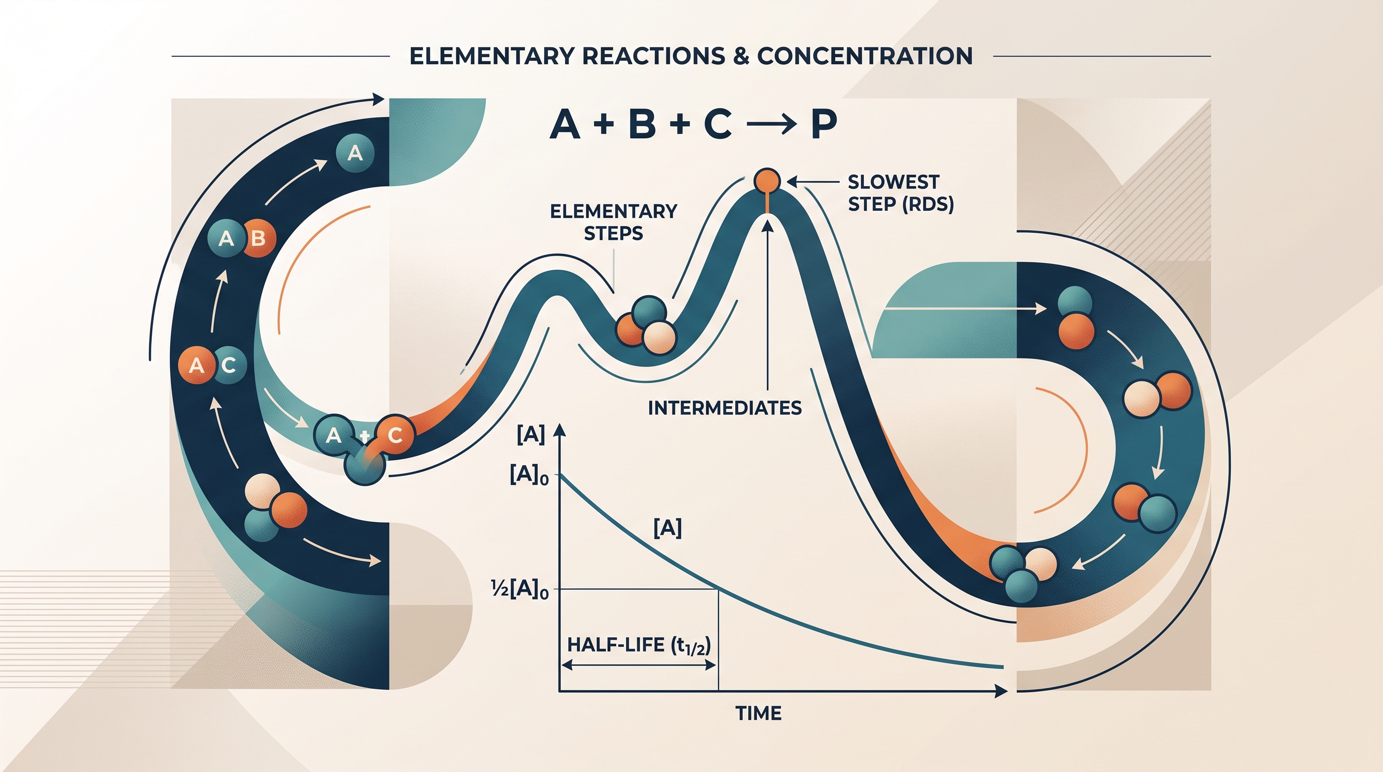
An elementary reaction is a single molecular event. Its rate law follows directly from the reacting particles in that step, unlike the experimentally determined rate law for an overall reaction, which may require evidence from several trials.

For a proposed mechanism, an intermediate is formed in one elementary step and consumed in a later step, so it cancels when the steps are added. A catalyst is consumed in an early step and regenerated later; it participates in the mechanism but does not appear in the net reaction.

The rate-determining step is the slow step that limits the overall rate. A valid mechanism must satisfy two tests: its elementary steps must add to the observed overall equation, and its predicted rate behavior must agree with the experimentally constructed rate law. A mechanism that balances atoms but predicts the wrong dependence on concentration is rejected.

For example, consider

$$ A+B\longrightarrow I $$

followed by

$$ I+C\longrightarrow P. $$

Here $I$ is an intermediate because it is produced and then consumed. Adding the steps gives

$$ A+B+C\longrightarrow P. $$

The mechanism must be checked against the measured rate law rather than accepted from stoichiometric balancing alone.

Science Practice 5: Mathematical Routines is central to Topics 5.3 and 5.4: transform data, calculate slopes and half-lives, track units, and use equations to test mechanisms. Science Practice 3: Representing Data and Phenomena also enters whenever concentration changes, spectrophotometric measurements, graphs, or mechanism diagrams are translated into chemical meaning.

Energy profiles for mechanisms are constructed and analyzed with the reaction-energy ideas developed in 5.6 Reaction Energy Profile; here, the essential mechanistic task is identifying elementary steps, intermediates, catalysts, and the rate-determining step without confusing a proposed pathway with experimental proof.

Retrieval check: A plot of $1/[A]$ versus time is linear with slope $0.080\ \mathrm{M^{-1},s^{-1}}$. What is the reaction order, and what happens to $[A]$ after one half-life? Answer: It is second order, $k=0.080\ \mathrm{M^{-1},s^{-1}}$, and the concentration becomes one-half its initial value; unlike a first-order reaction, successive second-order half-lives are not generally equal.