From the free course AP Macroeconomics on Lykke
3.7 Long-Run Self-Adjustment
Key concepts: Long-run self-adjustment in the AD-AS model · Recessionary gaps and below-full-employment output · Downward pressure on nominal wages and input prices · Inflationary expectations and their effect on SRAS · Rightward shifts of the short-run aggregate supply (SRAS) curve · Restoration of full employment and potential output · Effects of shifts in aggregate demand on output and the price level · Using economic concepts and models to determine outcomes
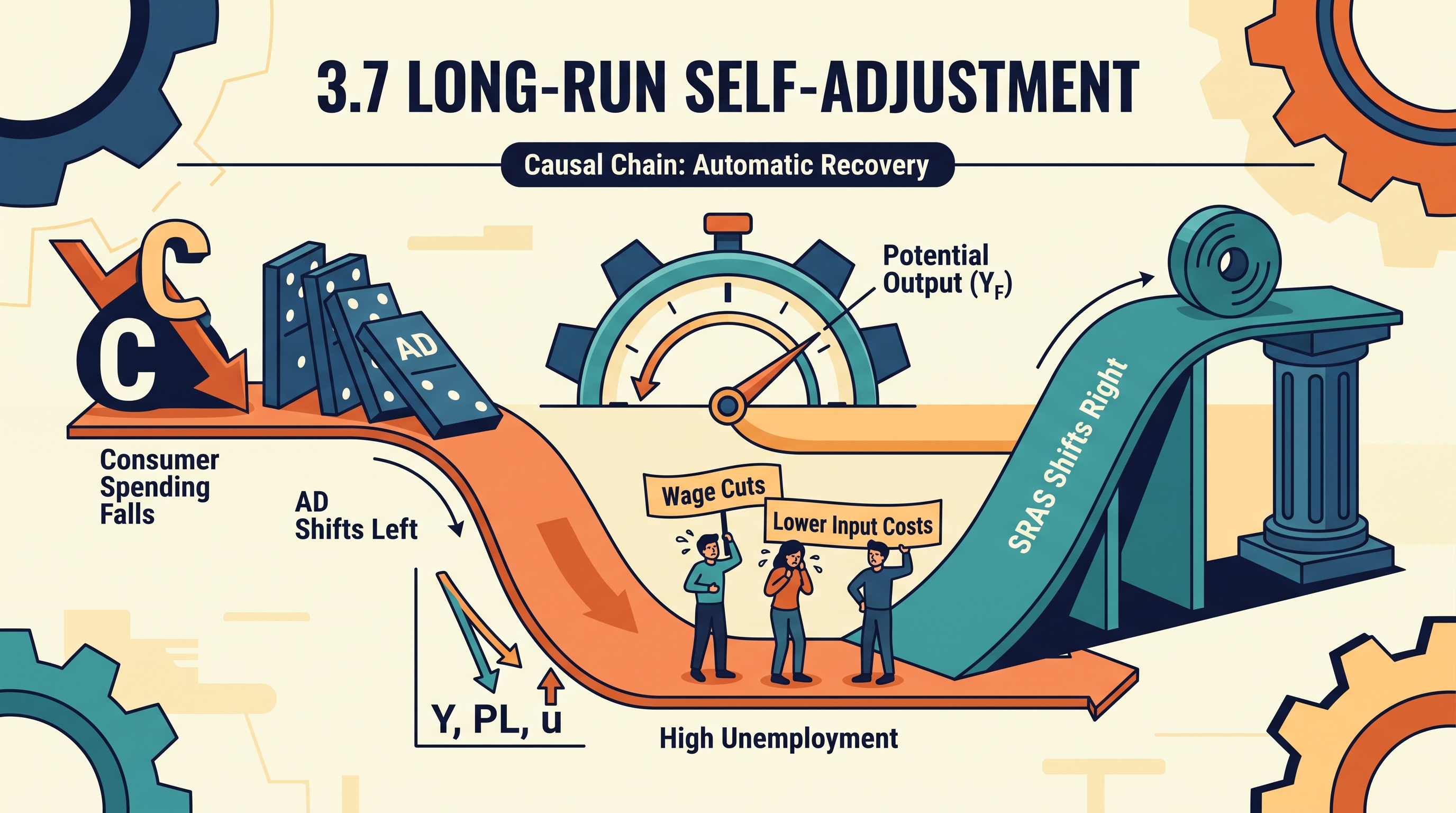
A recessionary gap does not necessarily last forever: when real output falls below the economy’s full-employment level, persistent unemployment can gradually lower firms’ input costs and shift short-run aggregate supply rightward until potential output is restored.
3.7 Long-Run Self-Adjustment
A recessionary gap does not necessarily last forever: when real output falls below the economy’s full-employment level, persistent unemployment can gradually lower firms’ input costs and shift short-run aggregate supply rightward until potential output is restored.
Investigative question: If a fall in consumer spending shifts aggregate demand left, why might the economy eventually return to full employment without a new policy action—and why would the final price level be lower?
CED alignment: Enduring Understanding MOD-2; Learning Objective MOD-2.I; Essential Knowledge MOD-2.I.1 and MOD-2.I.2; Suggested Skill 3.A: Manipulation — Determine the outcome of an economic situation using economic concepts, principles, or models.
From an AD shock to a recessionary gap
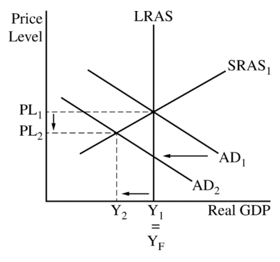
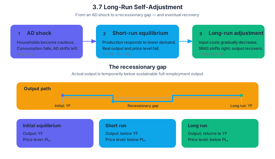
Suppose households suddenly become cautious and reduce consumption. Because consumption is part of aggregate demand, the AD curve shifts left. In the short run, the economy moves to a new equilibrium with both a lower price level and lower real output.
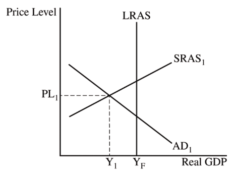
A recessionary gap exists when actual real output is below the full-employment or potential-output level, written as $Y_F$. The economy is producing less than it could when its labor and other resources are employed at sustainable full-employment levels.
The crucial distinction is between the immediate result and the later adjustment:
| Stage | Output | Price level | Main mechanism |
|---|---|---|---|
| Initial equilibrium | $Y_F$ | $PL_1$ | Economy is at full employment |
| Short run after AD shifts left | Below $Y_F$ | Below $PL_1$ | Lower spending reduces production |
| Long run | Returns to $Y_F$ | Below $PL_1$ | Lower input costs shift SRAS right |
Why unemployment changes costs
In the recessionary gap, firms sell less and reduce production. They need fewer workers, so unemployment rises. If unemployment remains high, workers have less bargaining power and nominal wages—wages measured in current dollars—face downward pressure. Other input prices may also decline as firms reduce their demand for materials, energy, transportation, and rented capital.
Lower input prices reduce firms’ per-unit production costs. At every possible price level, firms can now profitably produce more output. Economically, this is an increase in SRAS, represented by a rightward shift of the short-run aggregate supply curve.
Inflationary expectations also matter
The adjustment is not limited to wages and physical inputs. Inflationary expectations are what households and firms anticipate about future inflation. If a prolonged recession causes people to expect lower inflation, workers may negotiate smaller wage increases and firms may set lower prices. Those expectations reduce cost pressures and can also shift SRAS rightward.
The process continues in stages: lower output creates unemployment; unemployment places downward pressure on nominal wages and other input prices; lower costs increase SRAS; and the new equilibrium produces more real output. The adjustment stops when output returns to $Y_F$.
The final price level is lower
Imagine that consumer spending first shifts $AD_1$ leftward. The economy lands at a short-run equilibrium below $Y_F$, creating a recessionary gap. As SRAS shifts right, the economy moves along the unchanged AD curve toward $Y_F$.
Because the new intersection occurs farther down the downward-sloping AD curve, the final equilibrium price level is less than the initial level $PL_1$. Output returns to full employment, but the price level does not return to its original value.
Key result: After long-run self-adjustment from a recessionary gap, real output returns to $Y_F$, while the final price level is below the initial price level $PL_1$.
This result depends on identifying the correct curve shift. The original decline in consumer spending shifts AD left. The later response to unemployment and falling costs shifts SRAS right. LRAS does not shift merely because the economy is in a recession; a shift in LRAS represents a change in full-employment output or economic growth, as specified by MOD-2.I.2.
Misconception check: “The recession fixes itself by shifting AD back”
Misconception: Students often draw AD shifting right during self-adjustment. That would mean aggregate demand has recovered, but self-adjustment describes a change in production costs and expectations. Therefore, the correct movement is a rightward shift of SRAS, not AD.
A second misconception is that returning to full employment means returning to the original price level. It does not. With AD unchanged, a rightward SRAS shift restores $Y_F$ at a lower price level than $PL_1$.
Skill 3.A in action
To apply 3.A: Manipulation, trace the complete causal chain rather than naming only the first effect:
$$ C \downarrow \Rightarrow AD \text{ shifts left} \Rightarrow Y \downarrow,\ PL \downarrow \Rightarrow u \uparrow \Rightarrow \text{nominal wages and input prices} \downarrow \Rightarrow SRAS \text{ shifts right} \Rightarrow Y \to Y_F,\ PL < PL_1 $$
Retrieval check: An economy is initially at $Y_F$. Consumer confidence falls, shifting AD left. In the long run, what curve shifts, what causes that shift, and how does the final price level compare with the original price level? The complete answer is: SRAS shifts right because high unemployment lowers nominal wages, input costs, and possibly inflationary expectations; output returns to $Y_F$, and the final price level is below the original $PL_1$.
Source Materials
- AP Macroeconomics Course and Exam Description
- AP Macroeconomics Course and Exam Description Clarifications and Corrections
- AP Macroeconomics Course Overview
- AP Macroeconomics Course at a Glance
- AP Macroeconomics Course at a Glance Poster
- AP Macroeconomics
- AP Macroeconomics
- AP Macroeconomics Sample Syllabus 1
- (b)(i) Explain that input prices (e.g., nominal wages) and/or inflationary expectations will decrease, causing SRAS to increase until it reaches full employment.
- For the second point, the graph must show a rightward shift in the demand curve for the
- For the second point, the graph must show a rightward shift in the demand curve for the
- For the second point, the graph must show a rightward shift in the demand curve for the