From the free course AP Macroeconomics on Lykke
3.5 Equilibrium in the Aggregate Demand–Aggregate Supply (AD–AS) Model
Key concepts: Aggregate Demand–Aggregate Supply (AD–AS) model · Equilibrium in the AD–AS model · Aggregate demand · Aggregate supply · Macroeconomic indicators · Gross domestic product (GDP) · Real GDP · GDP deflator · Movement along a curve versus shifts of a curve · Accurately labeled economic graphs
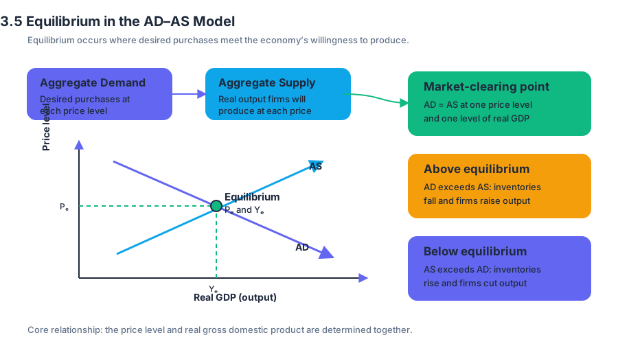
The AD–AS model shows how an economy’s overall price level and real output are determined together. Its central question is simple: Where do the economy’s desired purchases meet the economy’s willingness to produce?
3.5 Equilibrium in the Aggregate Demand–Aggregate Supply (AD–AS) Model
The AD–AS model shows how an economy’s overall price level and real output are determined together. Its central question is simple: Where do the economy’s desired purchases meet the economy’s willingness to produce?
Learning Objective MOD-3.E: Explain how equilibrium in the aggregate demand–aggregate supply model represents an economy’s performance. Essential Knowledge MOD-3.E.1: The AD–AS model represents the relationship between the price level and real gross domestic product.
Reading the AD–AS equilibrium
Aggregate demand, or $AD$, is the total quantity of domestically produced final goods and services demanded at different price levels. It combines consumption, investment, government spending, and net exports:
$$AD = C + I + G + NX$$
Aggregate supply describes the total quantity of goods and services firms are willing and able to produce at different price levels. In the short run, the relevant curve is short-run aggregate supply, or $SRAS$.
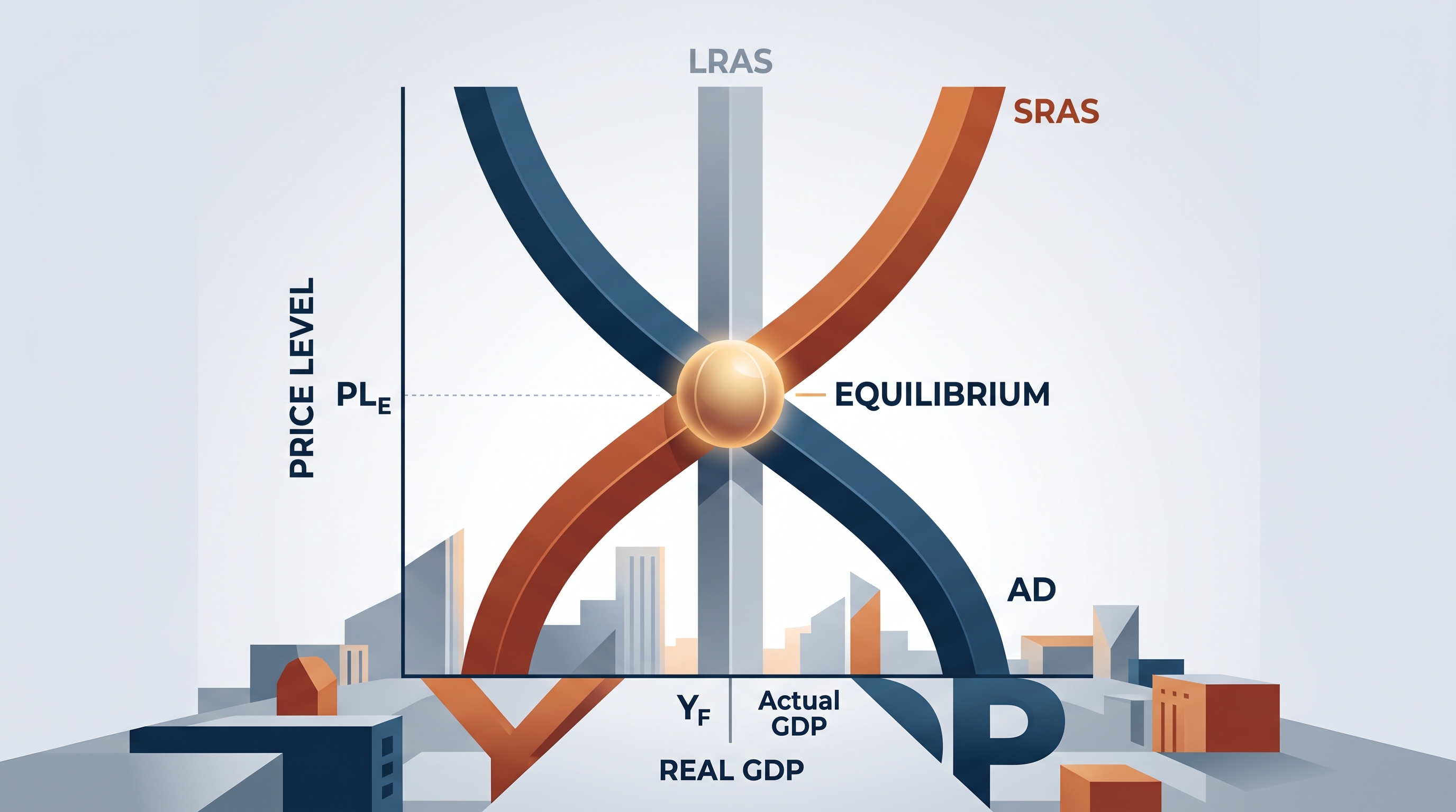
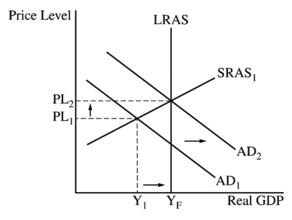
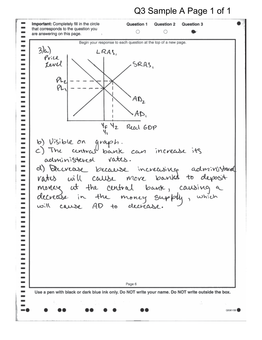
Equilibrium in the AD–AS model occurs where the $AD$ curve intersects the $SRAS$ curve. At that point, planned spending equals actual production.
The horizontal axis must measure real GDP, also written as real output $Y$. The vertical axis must measure the price level, often written as $PL$. The equilibrium intersection identifies both the economy’s current real output, such as $Y_1$, and its current price level, such as $PL_1$.
Businesses influence aggregate demand through investment and production decisions; the government affects it through purchases, taxes, and transfers; and the rest of the world affects it through exports, imports, exchange rates, and international income. The model therefore connects household, business, government, and international activity in one economy-wide picture.
Movement versus shift
A change in the price level causes a movement along an existing $AD$ or $SRAS$ curve. A change in one of the determinants other than the price level causes the entire curve to shift.
| Change | Graphical result | Example |
|---|---|---|
| Price level rises | Movement upward along $AD$ | Households purchase less real output because purchasing power and interest-sensitive spending change |
| Consumption changes for a reason other than $PL$ | Shift of $AD$ | Consumer confidence increases |
| Input prices change | Shift of $SRAS$ | Energy costs rise |
| Price level falls | Movement downward along $SRAS$ | Firms respond to the lower overall selling-price level |
Misconception check — “Any change in output shifts $AD$.” Not necessarily. If the price level changes and the economy moves to another point on the same curve, that is a movement along the curve. A shift requires a change in a determinant such as consumption, investment, government spending, net exports, resource prices, or productivity.
Using macroeconomic indicators
The equilibrium output shown in the model is measured with real GDP, which values current production using prices from a base year. Real GDP is therefore designed to measure changes in production while removing the effect of changing prices. Nominal GDP uses current prices, so it can rise because the economy produces more, prices rise, or both.
The GDP deflator measures the price level of all final goods and services included in GDP:
$$GDP\ deflator = \frac{Nominal\ GDP}{Real\ GDP} \times 100$$
For example, suppose nominal GDP is $$1{,}200$ billion and real GDP is $$1{,}000$ billion. Then:
$$GDP\ deflator = \frac{1{,}200}{1{,}000}\times100 = 120$$
A deflator of $120$ means that the prices of domestically produced final goods and services are $20%$ higher than in the base year. It does not mean that real output is $20% higher.
Gaps and the business cycle
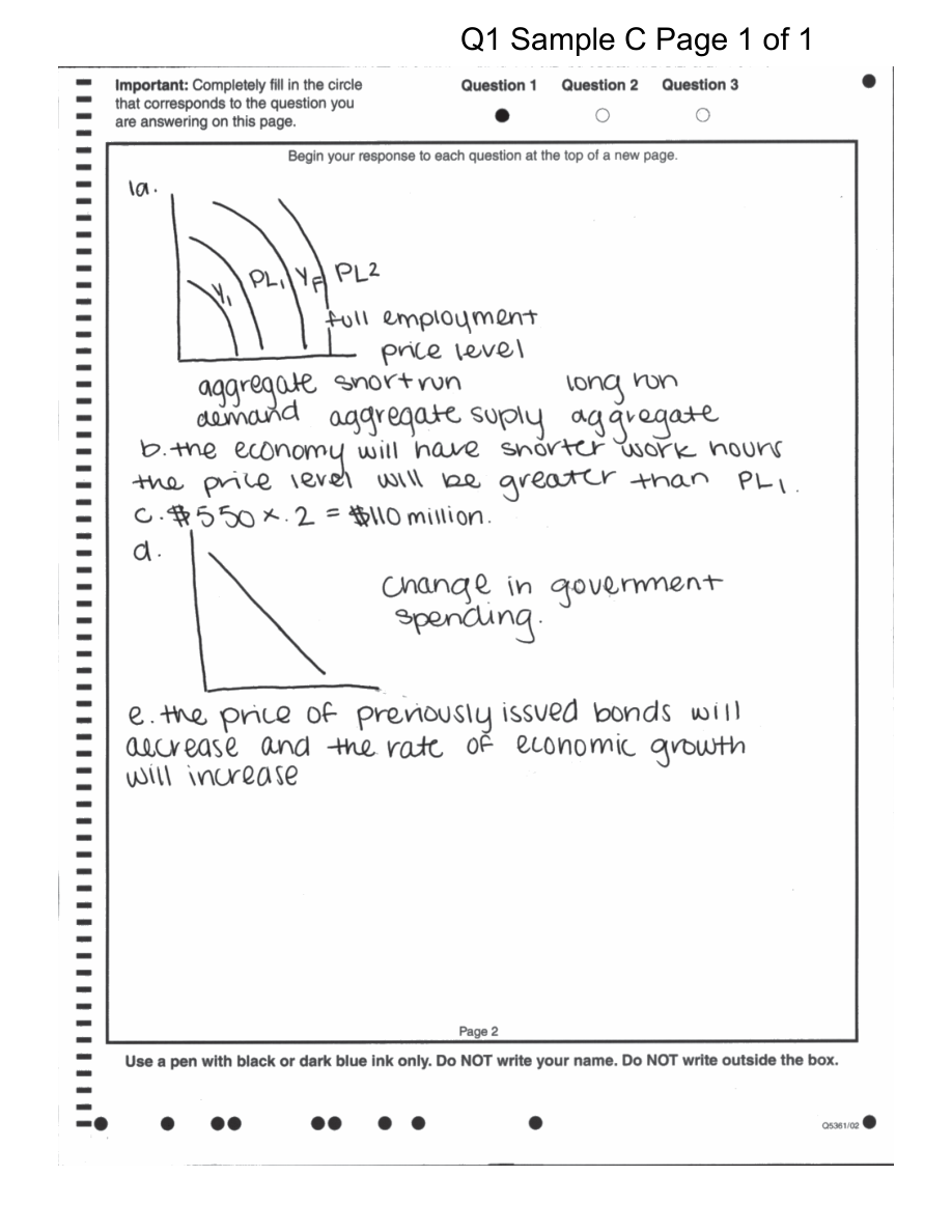
Using the LRAS benchmark from Section 3.4, compare the AD–SRAS equilibrium output with full-employment output $Y_F$. If equilibrium output is below $Y_F$, the economy has a recessionary gap and typically elevated cyclical unemployment. If equilibrium output is above $Y_F$, it has an inflationary gap, meaning short-run output exceeds its full-employment benchmark.
Suppose an economy’s equilibrium is at $Y_1$, while the benchmark is $Y_F$, with $Y_1>Y_F$. The graph identifies an inflationary gap; macroeconomic indicators would likely show output above sustainable full-employment production and pressure on the price level. If instead $Y_1<Y_F$, the economy is operating below capacity, consistent with a downturn in the business cycle.
Worked interpretation: A decline in business investment reduces one component of $AD$. On the graph, locate the new $AD$–$SRAS$ intersection and read the two coordinates: the new equilibrium real GDP and price level. The correct explanation must include the causal chain: lower investment $\rightarrow$ lower aggregate demand $\rightarrow$ lower equilibrium real output and price level, assuming an unchanged $SRAS$ curve.
AP reasoning and retrieval check
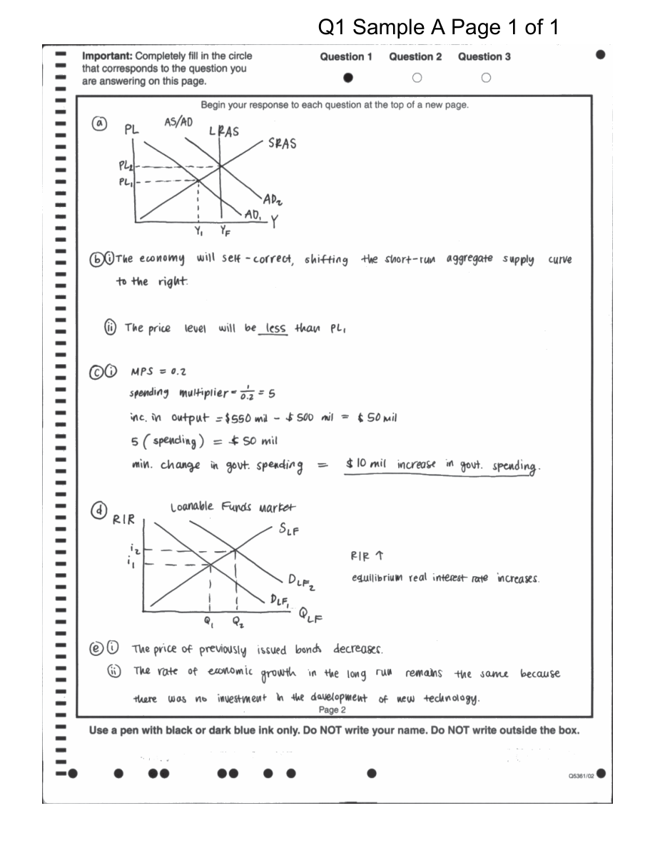
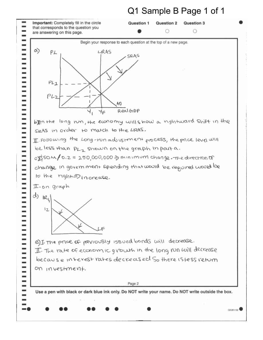
This topic directly develops Skill Category 1: Principles and Models, especially defining and explaining the AD–AS model; Skill Category 2: Interpretation, by reading GDP, real GDP, and the GDP deflator; and Skill Category 4: Graphing and Visuals, especially MOD-2.A.2 and MOD-2.A.3, which require an accurately labeled economic graph and an explanation of the relationship represented. The graph must show $PL$ and real GDP on the axes, correctly labeled $AD$ and $SRAS$ curves, and a clearly marked equilibrium.
Retrieval check: If nominal GDP rises while real GDP remains constant, what must happen to the GDP deflator? If the $AD$–$SRAS$ intersection lies left of $Y_F$, name the gap and the likely business-cycle condition.

Source Materials
- AP Macroeconomics Course and Exam Description
- AP Macroeconomics Course and Exam Description Clarifications and Corrections
- AP Macroeconomics Course Overview
- AP Macroeconomics Course at a Glance
- AP Macroeconomics Course at a Glance Poster
- AP Macroeconomics
- AP Macroeconomics
- AP Macroeconomics Sample Syllabus 1
- Figure — Sample Responses Q1 - Set 1 (p. 3)
- Figure — Sample Responses Q1 - Set 1 (p. 5)
- Figure — Sample Responses Q1 - Set 1 (p. 6)
- Figure — Sample Responses Q1 - Set 1 (p. 7)