3.2 Multipliers

3.2 Multipliers

A $1 increase in spending can raise total real GDP by more than $1 because one person’s spending becomes another person’s income, which creates further rounds of spending. This chain reaction is the multiplier effect.

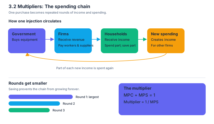
The spending chain

Imagine that the government purchases $100 million of new public-transport equipment. The firms producing the equipment receive that $100 million as revenue and pay some of it to workers and suppliers. Those recipients spend part of their new income, creating income for others, who spend part of that income again.

The first round is always the largest. Each later round is smaller because households save part of their income rather than spend all of it. The marginal propensity to consume, or $MPC$, is the fraction of an additional dollar of disposable income that households spend; the marginal propensity to save, or $MPS$, is the fraction saved.

$$MPC + MPS = 1$$

If households spend $0.80 of every additional dollar, then $MPC = 0.8$ and $MPS = 0.2$. The spending multiplier is therefore:

$$\text{Spending multiplier} = \frac{1}{1-MPC} = \frac{1}{MPS}$$

$$\text{Spending multiplier} = \frac{1}{1-0.8} = \frac{1}{0.2}=5$$

Worked example: government purchases

Suppose real GDP is below potential output by $12$ billion. The government increases purchases by $3$ billion, and the economy’s $MPC$ is $0.75$.

$$\text{Spending multiplier}=\frac{1}{1-0.75}=4$$

$$\Delta \text{Real GDP}=4 \times $3\text{ billion}=$12\text{ billion}$$

The initial $3$-billion increase in government purchases produces a total $12$-billion increase in real GDP, exactly closing the output gap in this simplified model. The rounds are:

Spending round	New spending
Initial government purchases	$$3.00$ billion
Round 2: $0.75 \times $3.00$	$$2.25$ billion
Round 3: $0.75 \times $2.25$	$$1.69$ billion
Later rounds	progressively smaller
Total effect	$$12.00$ billion

In a complete macroeconomic model, the final effect may be smaller because households may save, taxes may reduce disposable income, imports may send spending abroad, and higher interest rates may reduce private investment. The multiplier is therefore a calculated model result, not a guarantee that every dollar produces the same final increase.

Tax changes use a different multiplier

A tax change affects GDP indirectly. When taxes fall, disposable income rises; households then spend only the fraction represented by the $MPC$. Consequently, the tax multiplier is smaller in absolute value than the spending multiplier:

$$\text{Tax multiplier}=\frac{-MPC}{1-MPC}$$

With $MPC=0.75$:

$$\text{Tax multiplier}=\frac{-0.75}{0.25}=-3$$

A tax cut of $$4$ billion changes real GDP by:

$$\Delta \text{Real GDP}=(-3)(-$4\text{ billion})=$12\text{ billion}$$

The negative sign means that a tax increase decreases aggregate demand, while a tax cut increases it. Notice that a $$4$-billion tax cut and a $$3$-billion increase in government purchases have the same total effect in this example, because government purchases enter aggregate demand directly but tax changes first pass through household spending.

Key insight: For an equal-sized change, the government-purchases multiplier is larger than the tax multiplier because households do not spend all of a tax change.

AP skills in action

Topic identifier: 3.2 Multipliers. This topic is assessed through the official skill categories Skill Category 1: Principles and Models, Skill Category 2: Interpretation, Skill Category 3: Manipulation, and Skill Category 4: Graphing and Visuals.

• Skill Category 1: Principles and Models: identify whether a policy changes government purchases, taxes, or another component of spending, then select the appropriate multiplier.
• Skill Category 2: Interpretation: explain why successive rounds of spending become smaller and connect the result to changes in real GDP.
• Skill Category 3: Manipulation: calculate $MPC$, $MPS$, the spending multiplier, the tax multiplier, or the required policy change.
• Skill Category 4: Graphing and Visuals: show the resulting shift in aggregate demand and identify the change in equilibrium real GDP when a multiplier problem supplies an AD–AS diagram.

Misconception check

Misconception: “The multiplier is always larger than $1$.” The spending multiplier exceeds $1$ only when $0<MPC<1$. A larger $MPC$ produces a larger multiplier because less income leaks into saving. Also, the tax multiplier is negative, not positive: a tax increase reduces disposable income and decreases aggregate demand.

Retrieval check

If $MPC=0.6$ and government purchases rise by $$5$ billion, calculate the change in real GDP.

$$\text{Spending multiplier}=\frac{1}{1-0.6}=2.5$$

$$\Delta \text{Real GDP}=2.5 \times $5\text{ billion}=\boxed{$12.5\text{ billion}}$$