3.6 Changes in the AD–AS Model in the Short Run

3.6 Changes in the AD–AS Model in the Short Run

A recessionary gap exists when an economy’s actual output is below its potential output, so firms produce less and employ fewer workers than they would at full employment. The AD–AS model makes this gap visible by comparing the short-run equilibrium output with the economy’s sustainable capacity.

The time horizons: short run versus long run

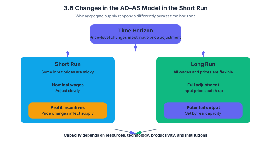
In the short run, some input prices—especially nominal wages—are sticky, meaning they do not adjust immediately when economic conditions change. Because firms’ costs are temporarily fixed, a change in the price level can change firms’ profit incentives and the quantity of output they supply.

In the long run, all wages and prices are flexible. Once input prices fully adjust, changes in the overall price level no longer change the economy’s real productive capacity. Potential output depends instead on resources, technology, productivity, and institutions.

Why SRAS slopes upward

The short-run aggregate supply (SRAS) curve shows the relationship between the price level and the quantity of goods and services supplied in an economy (MOD-2.C.1). It slopes upward because wages and other prices are sticky in the short run (MOD-2.C.2): if firms can sell output at higher prices while their input costs have not risen proportionally, production becomes more profitable.

A movement along SRAS is caused by a change in the price level. A shift of SRAS is caused by a change in production costs (MOD-2.C.3). For example, higher expected inflation may lead workers to negotiate higher nominal wages. Higher wages raise firms’ costs, shifting SRAS left; lower wages or lower inflationary expectations reduce costs, shifting SRAS right.

Named misconception — “Every change in output shifts SRAS.” A change in the price level causes movement along a given SRAS curve. A change in wages, resource prices, productivity, taxes on production, or inflationary expectations shifts the entire curve.

LRAS and the two kinds of equilibrium

The long-run aggregate supply (LRAS) curve is vertical at potential output, labeled $Y_F$. Its vertical shape shows that a long-run change in the price level does not change real output: once wages and prices adjust fully, the economy returns to its productive capacity.

Short-run equilibrium occurs where $AD$ intersects $SRAS$. Long-run equilibrium occurs where $AD$ intersects $LRAS$ at potential output, $Y_F$, with wages and prices fully adjusted. Thus, an economy can have a short-run equilibrium at an output level different from $Y_F$, but long-run equilibrium requires actual output to equal potential output.

If short-run equilibrium output is $Y_1$ and $Y_1<Y_F$, the economy has a recessionary gap. If output exceeds $Y_F$, it has an inflationary gap. The gap is measured horizontally on the AD–AS graph as the difference between actual output and potential output.

Shocks, output, prices, and employment

Macroeconomic changes affect output, the price level, and employment in both the short run and the long run, although the immediate effects can differ from the eventual capacity of the economy.

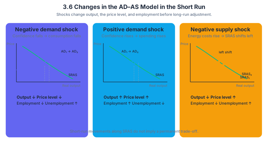
Suppose consumer confidence falls. Consumption decreases, so aggregate demand shifts left from $AD_1$ to $AD_2$. In the short run, the new intersection with SRAS produces lower real output and a lower price level. Firms need fewer workers, so employment falls and cyclical unemployment rises.

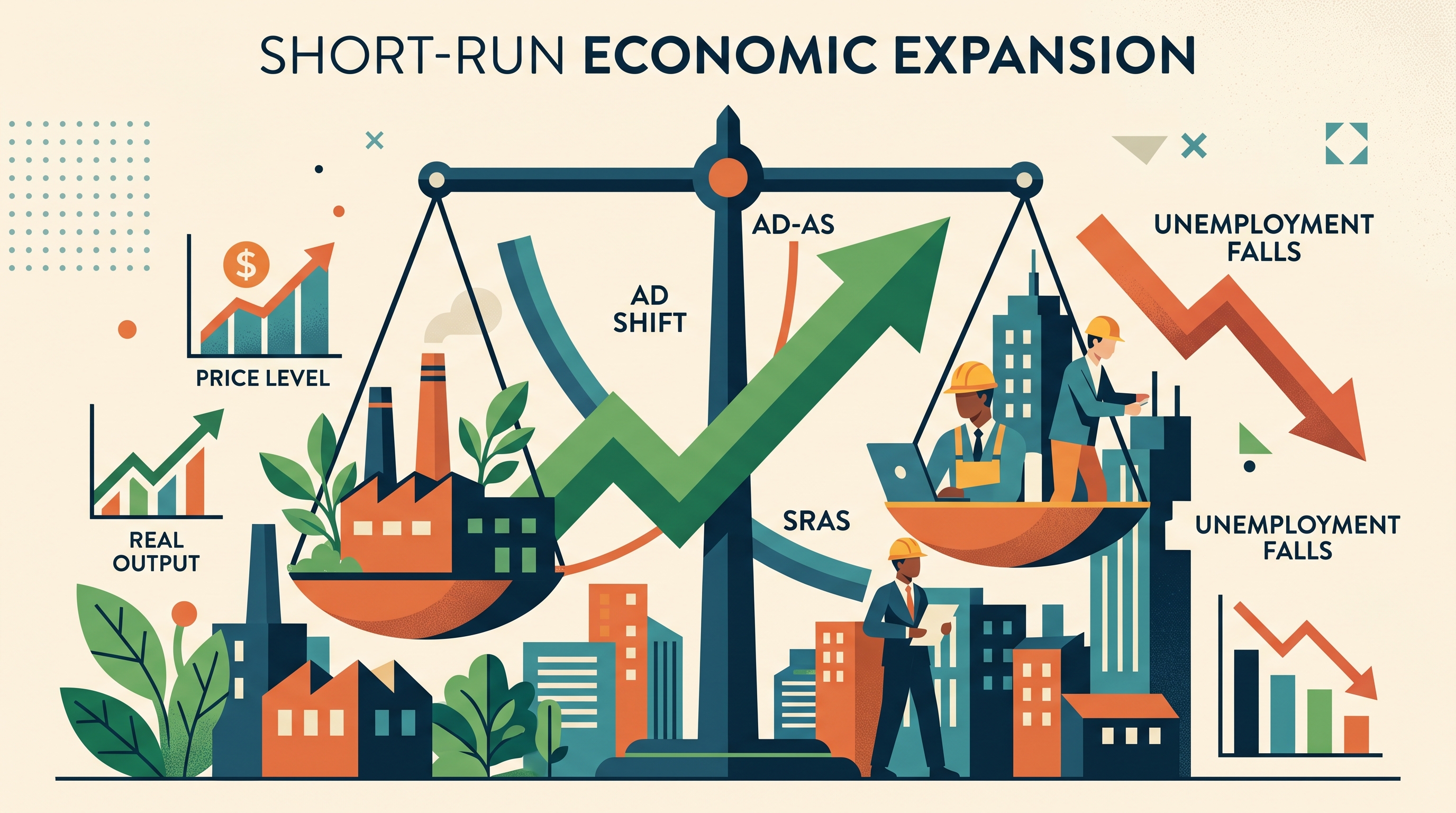
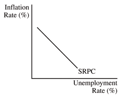
A positive demand shock works in the opposite direction: $AD$ shifts right, increasing both the short-run price level and real output. Higher output requires more labor, so employment rises and unemployment falls. This movement along SRAS illustrates the short-run inverse relationship between inflation and unemployment identified in MOD-2.D.1, without implying that the trade-off lasts permanently.

A supply shock has a different signature. If energy prices rise, firms face higher production costs and SRAS shifts left. The economy experiences a lower level of output and a higher price level at the same time—a combination often called stagflation. Because employment is tied to production, unemployment tends to rise as well.

Peaks, troughs, and output gaps

A business-cycle peak is the turning point at which an expansion ends and the economy begins contracting. A trough is the turning point at which a contraction ends and a new expansion begins.

On a time graph of actual output, a peak is the highest point before output turns downward, while a trough is the lowest point before output turns upward. A recessionary gap can occur during a contraction when actual output falls below potential output, even though potential output itself may continue growing.

Worked example: reading an AD–AS shock

An economy begins with $Y_1=950$ billion and potential output of $Y_F=1{,}000$ billion. The recessionary gap is

$$ Y_F-Y_1=1{,}000-950=$50\text{ billion}. $$

If a decline in investment shifts $AD$ left, the short-run result is lower real output, a lower price level, and higher cyclical unemployment. The graph should show $AD$ shifting left while $SRAS$ and vertical $LRAS$ remain in place; the new short-run equilibrium lies left of $Y_F$.

Graphing skill 3.C: “Create a correctly labeled graph or visual to represent an economic model or market.” For an AD–AS response, label the vertical axis Price Level, the horizontal axis Real Output or Real GDP, draw downward-sloping $AD$, upward-sloping $SRAS$, and vertical $LRAS$ when long-run capacity is relevant. Mark the initial and final equilibria and use arrows to show every curve shift.

Retrieval check

An economy’s $AD$ curve shifts right while SRAS remains unchanged. What happens in the short run to real output, the price level, employment, and unemployment? Answer: real output, the price level, and employment rise; unemployment falls. If the new output exceeds $Y_F$, the economy has an inflationary gap.