4.1 Linear Momentum

4.1 Linear Momentum

A rolling wheel can translate across the floor while rotating about its center, so its motion carries two linked descriptions: linear momentum for the motion of its center of mass and angular motion for its spin. The key is to connect these descriptions without assuming that they are literally the same quantity.

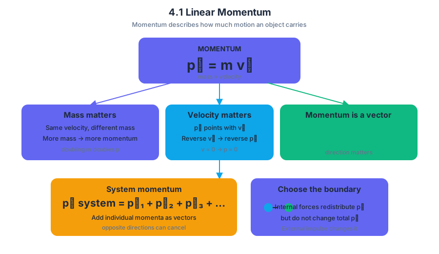
Linear momentum is the product of an object's mass and velocity:

$$\vec{p}=m\vec{v}$$

Momentum is a vector, so its direction is the direction of the velocity. Its SI unit is $\mathrm{kg\cdot m/s}$.

Momentum as “mass in motion”

A heavy cart and a light cart moving at the same velocity do not have the same momentum. Doubling the mass doubles the momentum; reversing the velocity reverses the momentum. A stationary object has zero linear momentum because $v=0$, even though it still has mass.

For a system of objects, total momentum is the vector sum of the individual momenta:

$$\vec{p}_{\text{system}}=\vec{p}_1+\vec{p}_2+\vec{p}_3+\cdots$$

The system boundary matters. Forces between objects inside the selected system can redistribute momentum within that system, but they do not change the system's total momentum by themselves. An external force can change the total momentum by exerting an impulse.

Force–time graphs reveal momentum change

The change in momentum is related to the net force acting over a time interval:

$$\Delta \vec{p}=\vec{F}_{\text{net}}\Delta t$$

For a force that varies with time, the change in momentum is estimated from the area under a force-versus-time graph:

$$\Delta \vec{p}\approx \text{area under the }F\text{-versus-}t\text{ graph}$$

For example, suppose a wheel experiences a horizontal force that rises linearly from $0$ to $12\ \mathrm{N}$ during $0.40\ \mathrm{s}$. The graph forms a triangle, so

$$\Delta p=\frac{1}{2}(0.40\ \mathrm{s})(12\ \mathrm{N})=2.4\ \mathrm{N\cdot s}$$

Because $\mathrm{N\cdot s}=\mathrm{kg\cdot m/s}$, the wheel's momentum changes by $2.4\ \mathrm{kg\cdot m/s}$ in the force's direction.

A graph must use a linear scale and clearly identified axes, including labels and units. A curved force graph is not averaged by simply using its highest value; its area must represent the accumulated effect of force over time.

Velocity–time graphs reveal kinetic-energy change

Momentum depends linearly on velocity, but translational kinetic energy depends on the square of velocity:

$$K=\frac{1}{2}mv^2$$

Thus, a velocity-versus-time graph can provide the initial and final speeds, which are then used to calculate the change in kinetic energy:

$$\Delta K=K_f-K_i=\frac{1}{2}m(v_f^2-v_i^2)$$

If a $2.0\ \mathrm{kg}$ cart changes speed from $3.0\ \mathrm{m/s}$ to $5.0\ \mathrm{m/s}$, then

$$\Delta K=\frac{1}{2}(2.0\ \mathrm{kg})\left[(5.0\ \mathrm{m/s})^2-(3.0\ \mathrm{m/s})^2\right]$$

$$\Delta K=16\ \mathrm{J}$$

The slope of a velocity-versus-time graph gives acceleration, while the values of velocity determine kinetic energy. The area under that graph instead represents displacement, not kinetic-energy change.

Linear and angular quantities in rolling

A rolling rigid body has a center-of-mass velocity $v$ and an angular velocity $\omega$. For pure rolling—rolling without slipping—the contact point is instantaneously at rest relative to the surface, and

$$v=R\omega$$

where $R$ is the wheel's radius. The analogous quantities form a useful translation:

Linear quantity	Angular analogue
Position or displacement $x$	Angular position $\theta$
Velocity $v$	Angular velocity $\omega$
Acceleration $a$	Angular acceleration $\alpha$
Mass $m$	Rotational inertia $I$
Momentum $p=mv$	Angular momentum $L=I\omega$

These are analogous relationships, not interchangeable ones. For example, $p=mv$ describes linear momentum, whereas $L=I\omega$ describes angular momentum. The symbols play parallel roles, but mass is not rotational inertia and velocity is not angular velocity.

A useful rolling investigation plots measured $v$ against measured $\omega$ for wheels of the same radius. From $v=R\omega$, the graph should be linear:

$$v=R\omega$$

If $v$ is on the vertical axis and $\omega$ is on the horizontal axis, the slope is

$$\text{slope}=\frac{\Delta v}{\Delta\omega}=R$$

For data with slope $0.080\ \mathrm{m}$, the wheel's radius is $R=0.080\ \mathrm{m}$. The graph therefore turns simultaneous linear and angular measurements into a physical measurement of radius. Clear axis labels and units are essential.

Rolling while slipping

Pure rolling is a special condition, not the definition of all rolling. During rolling while slipping, the wheel rotates and its center moves, but the contact point slides across the surface. Therefore $v$ and $\omega$ must be treated independently; the relation $v=R\omega$ does not apply during the slipping interval.

Kinetic friction acts at the contact region. Its effect is qualitative but predictable: it decreases the linear speed and changes the angular speed until the pure-rolling condition is reached. The exact time and distance of this transition are beyond the required model here, but the linked change in linear and angular quantities is essential.

Misconception check — “Friction always slows rotation.”

Friction opposes the relative slipping at the contact point, not automatically the wheel's angular velocity. Depending on whether the wheel spins too quickly or translates too quickly for pure rolling, friction can decrease or increase $\omega$ while also changing $v$.

A strong explanation identifies what is observed, states the expected relationship, and then connects the two logically: slipping means $v\neq R\omega$; kinetic friction changes the translational and rotational motion; the difference shrinks until $v=R\omega$.

Retrieval check

A wheel's graph of $v$ versus $\omega$ has slope $0.25\ \mathrm{m}$. What quantity does the slope represent? If the wheel is slipping, may you use $v=R\omega$ at that instant? Answer: the slope represents radius, $R=0.25\ \mathrm{m}$; no, the pure-rolling relation applies only when there is no slipping.