AP Practice 6

AP Practice 6

A successful physics investigation turns a physical question into measurable evidence: identify the variables, design a procedure, represent the data, and use a physical model to justify a conclusion.

This practice targets an experimental design and analysis task, an exam task type that connects laboratory reasoning with the course’s three science practices: Science Practice 1: Creating Representations, Science Practice 2: Mathematical Routines, and Science Practice 3: Scientific Questioning and Argumentation.

Task: How does ramp angle affect the acceleration of a cart?

A student has a dynamics cart, a low-friction track, a motion sensor, a protractor, and a balance. The student wants to test the model that the cart’s acceleration down an inclined track depends on the component of gravitational force parallel to the track.

The student plans to vary the track angle $\theta$ and measure the cart’s acceleration $a$. For a simplified model with negligible friction,

$$ a = g\sin\theta $$

where $g$ is the local gravitational field strength.

Original practice prompt. Design an investigation that tests the model $a = g\sin\theta$. Your response should:

• identify the independent and dependent variables;
• describe how the data should be collected;
• specify a graph that could test the model;
• explain how the graph would support or challenge the model;
• identify one important source of uncertainty or systematic error;
• state how repeated trials improve the investigation.

Step 1: Build the experimental representation

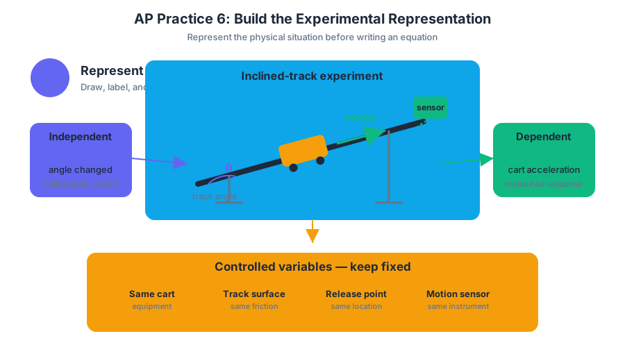
The first move is not to write an equation. It is to represent the physical situation clearly. Draw the inclined track, label the angle $\theta$, show the cart’s direction of motion, and identify the measured quantities.

The independent variable is the quantity deliberately changed: the angle $\theta$. The dependent variable is the quantity that responds and is measured: the cart’s acceleration $a$.

Useful controlled variables include the same cart, the same track surface, the same release location, and the same motion sensor. Keeping these features fixed helps ensure that changes in measured acceleration are associated with $\theta$, rather than with a different cart or altered friction.

Step 2: Design a reproducible procedure

A strong procedure might be:

1. Measure the track angle with a protractor and record $\theta$.
2. Place the cart at the same release position for every trial.
3. Release the cart without pushing it.
4. Use the motion sensor to obtain a velocity-versus-time graph.
5. Determine the slope of the best-fit line; this slope is the acceleration $a$.
6. Repeat the measurement several times for the same angle.
7. Repeat the entire process for several different values of $\theta$.

This procedure earns its strength from operational definitions. “Acceleration” does not mean merely that the cart is speeding up; here it is quantitatively defined as the slope of the velocity-versus-time graph:

$$ a = \frac{\Delta v}{\Delta t} $$

Science Practice 3: Scientific Questioning and Argumentation is visible in the testable question, the controlled procedure, and the planned evidence. A claim such as “steeper ramps produce greater acceleration” becomes scientific only when linked to measurements and a model.

Step 3: Choose the graph that tests the model

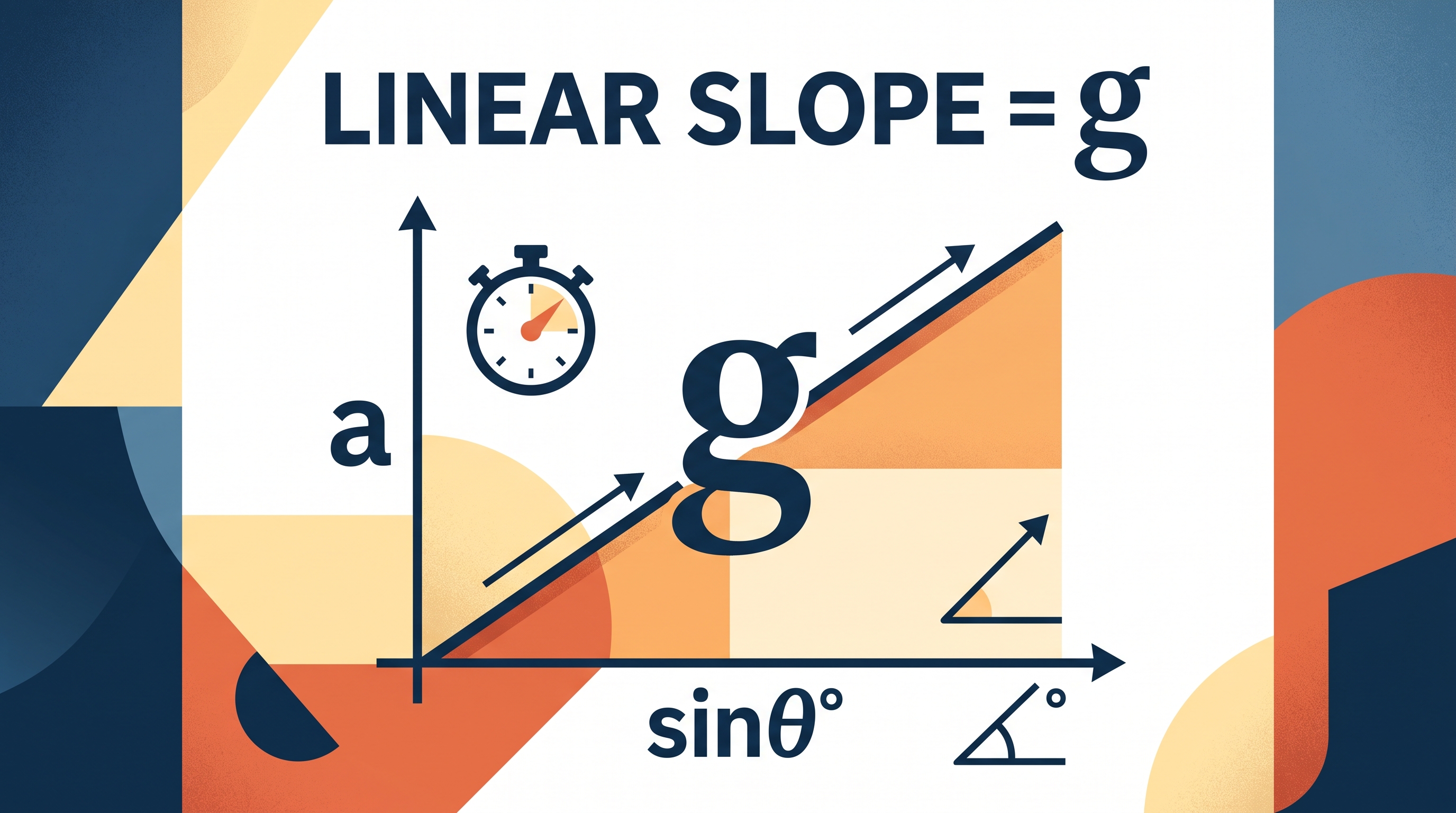
Because the model predicts $a = g\sin\theta$, the most direct graph is $a$ on the vertical axis versus $\sin\theta$ on the horizontal axis.

If the model is correct, the data should approximately form a straight line through the origin:

$$ a = g(\sin\theta) $$

The slope should be approximately $g$, with units of $\mathrm{m,s^{-2}}$.

This graph demonstrates Science Practice 1.B. Create quantitative graphs with appropriate scales and units, including plotting data. The horizontal axis must be labeled $\sin\theta$, which is dimensionless, and the vertical axis must be labeled $a$ in $\mathrm{m,s^{-2}}$. Plotting $a$ against $\theta$ directly may produce a curved relationship, so the transformed variable $\sin\theta$ is essential.

Step 4: Interpret evidence and uncertainty

Suppose the best-fit line has slope $8.7\ \mathrm{m,s^{-2}}$ and a small positive intercept. The slope is reasonably close to $g \approx 9.8\ \mathrm{m,s^{-2}}$, which supports the model, although friction may explain why the measured slope is smaller.

A positive intercept could indicate a systematic error, such as the motion sensor’s acceleration calibration or an incorrect estimate of the angle. A random release variation would instead cause trial-to-trial scatter without necessarily shifting every measurement in the same direction.

Repeating trials allows the student to estimate the spread in measured accelerations and identify anomalous results. Repetition does not automatically remove systematic error: measuring every angle incorrectly will produce consistently biased data.

What the examiner rewards

For this original, unofficial task, a high-scoring response would provide evidence aligned with the official practices and mathematical routines:

• 1.A. Create diagrams, tables, charts, or schematics to represent physical situations: a labeled ramp-and-cart diagram or organized data table.
• 1.B. Create quantitative graphs with appropriate scales and units, including plotting data: a graph of $a$ versus $\sin\theta$ with labels and units.
• 2.A. Derive a symbolic expression from known quantities by selecting and following a logical mathematical pathway: connect the predicted relation $a = g\sin\theta$ to the graph’s slope.
• 2.B. Calculate or estimate an unknown quantity with units from known quantities, by selecting and following a logical computational pathway: determine $g$ from the slope or calculate $a$ for a chosen angle.
• 3. Scientific Questioning and Argumentation: state a claim, cite the graph or measured values as evidence, and explain whether the evidence supports the model.

Timing and error review

Use approximately $12$–$15$ minutes for a first attempt: $2$ minutes to identify variables, $5$ minutes to design the procedure, $3$ minutes to select and explain the graph, and the remaining time to address uncertainty and repeated trials.

Afterward, classify each missed point as one of four errors: representation—the physical setup was unclear; mathematical—the model or slope was mishandled; experimental—a variable or uncertainty was overlooked; or argumentation—the claim was not connected to evidence. Then rewrite only the weakest response using a diagram, equation, or evidence statement.

Retrieval check

Why is $a$ plotted against $\sin\theta$ rather than directly against $\theta$? What physical meaning does the slope have if the model is correct?

Answer: The model predicts $a = g\sin\theta$, so $a$ versus $\sin\theta$ should be linear. The slope represents $g$, with units of $\mathrm{m,s^{-2}}$.