AP Practice 3

AP Practice 3

A strong physics investigation does more than produce a number: it connects a question, a controlled procedure, measured data, a mathematical model, and an evidence-based claim. This practice focuses on the free-response task type that asks you to design or analyze an experiment and defend a conclusion using representations, mathematical routines, and scientific argumentation.

Timing target: spend approximately $12$–$15$ minutes on one experimental-design or data-analysis task. Do not begin by calculating. First identify the physical relationship being tested, the variables that must be controlled, and the representation that will make the model visible.

The original investigation task

A student investigates how the period $T$ of a small-angle pendulum depends on its length $L$. The student has a pendulum, a meterstick, a stopwatch, and a digital balance. The pendulum bob is released from the same small angle for every trial.

The student measures the following values:

$L$ (m)	$T$ (s)
$0.25$	$1.00$
$0.40$	$1.27$
$0.60$	$1.56$
$0.90$	$1.91$
$1.20$	$2.20$

Task.

1. Design a graph that can test whether the model $T \propto \sqrt{L}$ is supported.
2. Describe one important procedure for reducing uncertainty in the period measurement.
3. Use the data to determine whether the model is reasonable.
4. Explain why the bob’s mass does not appear in the proposed model.

Step 1: Choose a representation that tests the model

The statement $T \propto \sqrt{L}$ is not tested most directly by plotting $T$ versus $L$. Instead, define a transformed variable:

$$ x=\sqrt{L} $$

If the model is correct, then

$$ T=k\sqrt{L} $$

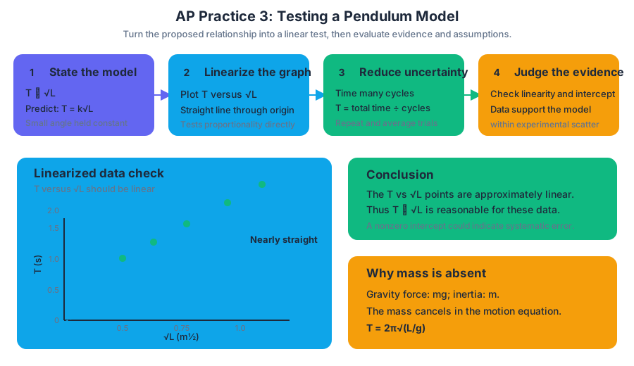
where $k$ is a constant. Therefore, a graph of $T$ on the vertical axis versus $\sqrt{L}$ on the horizontal axis should be approximately linear and should pass near the origin.

This response demonstrates Science Practice 1: Creating Representations, especially 1.B. Create quantitative graphs with appropriate scales and units, including plotting data, and 1.C. Create qualitative sketches of graphs that represent features of a model or the behavior of a physical system. A complete graph needs labeled axes, units, sensible scaling, plotted points, and a line or curve that represents the trend.

For the data, the transformed values are approximately:

$L$ (m)	$\sqrt{L}$ ($\text{m}^{1/2}$)	$T$ (s)
$0.25$	$0.50$	$1.00$
$0.40$	$0.63$	$1.27$
$0.60$	$0.77$	$1.56$
$0.90$	$0.95$	$1.91$
$1.20$	$1.10$	$2.20$

Step 2: Improve the measurement

A single stopwatch measurement includes the student’s reaction time when starting and stopping the timer. A better procedure is to measure the time for many complete oscillations, such as $10$ or $20$, and divide by the number of oscillations:

$$ T=\frac{t_{\text{total}}}{N} $$

Repeating this process and averaging the results further reduces the effect of random timing uncertainty. This is an example of Science Practice 3: Scientific Questioning & Argumentation, because the procedure is justified by the type of evidence needed to answer the question.

Step 3: Use the model to interpret the data

The transformed data give nearly constant values of $T/\sqrt{L}$:

$$ \frac{1.00}{0.50}=2.00\ \text{s},\text{m}^{-1/2} $$

$$ \frac{2.20}{1.10}=2.00\ \text{s},\text{m}^{-1/2} $$

The intermediate points produce values close to $2.00\ \text{s},\text{m}^{-1/2}$ as well. Thus, the graph of $T$ versus $\sqrt{L}$ would be approximately linear, supporting the model within experimental uncertainty.

This uses Science Practice 2: Mathematical Routines, specifically 2.A. Derive a symbolic expression from known quantities by selecting and following a logical mathematical pathway, 2.B. Calculate or estimate an unknown quantity with units from known quantities, by selecting and following a logical computational pathway, and 2.C. Compare physical quantities between two or more scenarios or at different times and locations in a single scenario.

Step 4: Explain the missing mass

For a small-angle pendulum, the period is modeled by

$$ T=2\pi\sqrt{\frac{L}{g}} $$

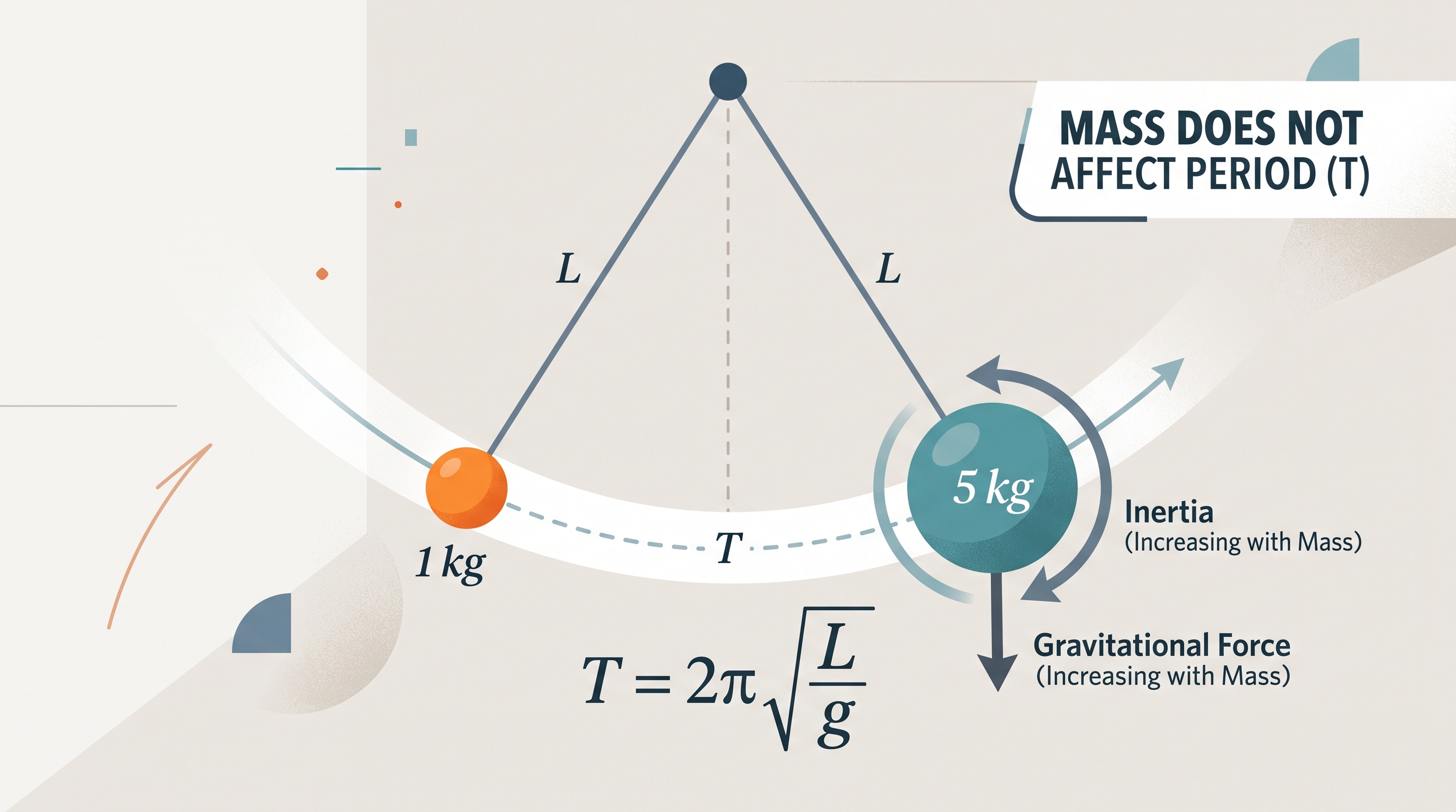
The bob’s mass does not appear because the gravitational force and the bob’s inertia both increase in proportion to mass. Their effects cancel in the equation of motion. A heavier bob may have a different air-resistance behavior, but in the ideal model its mass does not change the period.

Examiner-rewarded reasoning: identify the transformed graph, include units and scales, propose a procedure linked to uncertainty reduction, use data to support or reject the model, and justify the absence of mass from the governing relationship.

Named misconception — “More mass means a faster pendulum.” Mass can change the forces involved, but it also changes the inertia resisting acceleration by the same factor. For the ideal pendulum model, length and gravitational acceleration determine the period.

Error-review routine: after solving, check four items: Did the graph test the stated proportionality? Did the procedure control relevant variables? Did the conclusion cite data rather than merely assert agreement? Did every calculated quantity carry appropriate units?