From the free course AP Physics 1 on Lykke
AP Practice 4
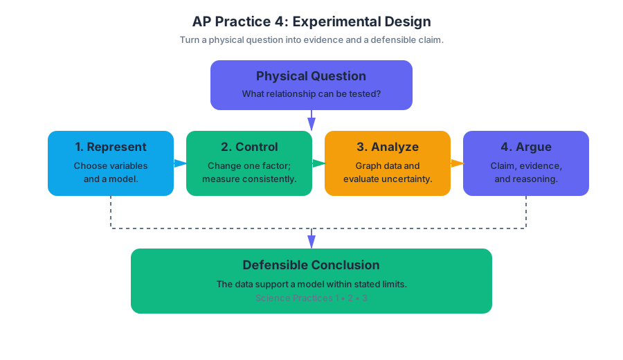
A strong experimental-design response does more than name an equation: it turns a physical question into measurable variables, a controlled procedure, evidence-based analysis, and a defensible claim.
AP Practice 4
A strong experimental-design response does more than name an equation: it turns a physical question into measurable variables, a controlled procedure, evidence-based analysis, and a defensible claim. In AP Physics 1, this task type especially exercises Science Practice 1: Creating Representations, Science Practice 2: Mathematical Routines, and Science Practice 3: Scientific Questioning & Argumentation.
The task type: experimental design and analysis
Treat the prompt as an investigation pipeline:
$$ \text{question} \longrightarrow \text{model} \longrightarrow \text{variables} \longrightarrow \text{procedure} \longrightarrow \text{data representation} \longrightarrow \text{claim} $$
The scoring opportunity is usually distributed across several kinds of reasoning: creating a useful diagram or graph, selecting measurable quantities, controlling variables, using mathematics consistently, and connecting the evidence to a physical principle. A response can lose credit even when its final equation is correct if the measurement plan cannot actually test the proposed relationship.
Original practice prompt
A student investigates how the period of a small-angle pendulum depends on its length. The student has a light string, several masses, a meterstick, a stopwatch, and a support stand. The pendulum is released from a small angle so that air resistance and the size of the angle can be treated as negligible.
Design an investigation that can be used to determine whether the period $T$ is proportional to the square root of the pendulum length $L$. Your response should include:
- a clearly identified independent variable, dependent variable, and at least two controlled variables;
- a procedure that produces repeatable measurements;
- a graph that could test the proposed relationship;
- a mathematical method for obtaining the proportionality constant;
- one source of uncertainty and one improvement.
Worked reasoning: what an examiner can reward
1. Build a physical representation
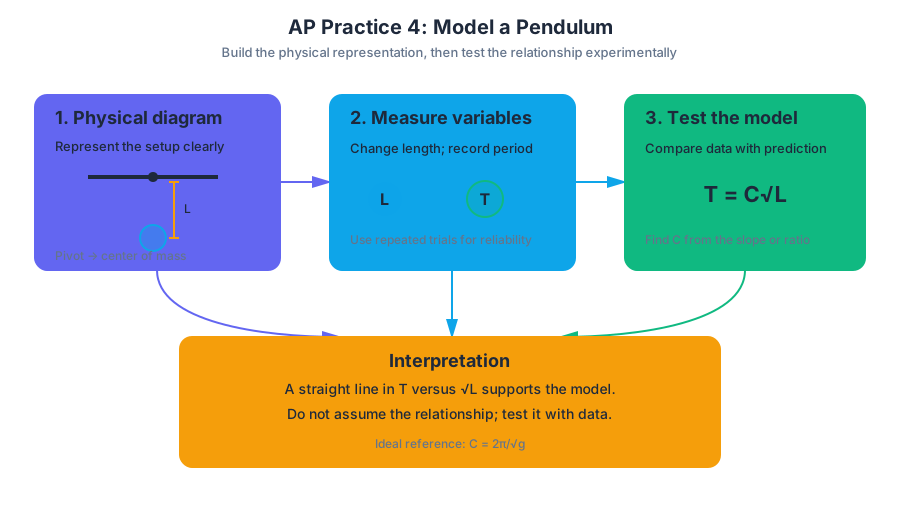
Draw the pendulum and label the length from the pivot to the center of the mass, not merely the length of exposed string. This diagram is a direct use of 1.A. Create diagrams, tables, charts, or schematics to represent physical situations.
The relevant model is
$$ T = C\sqrt{L}, $$
where $C$ is a constant for a particular location and pendulum setup. For an ideal small-angle pendulum, the model predicts $C = 2\pi/\sqrt{g}$, but the investigation should test the relationship experimentally rather than assume that the result is true.
2. Identify and control variables
The independent variable is pendulum length $L$. The dependent variable is period $T$. The student should keep the mass, release angle, string type, and pivot arrangement constant; at least two controls must be stated clearly. Keeping the release angle small matters because the model being tested applies to small oscillations.
3. Design repeatable measurements
Measure at least five different lengths. For each length, displace the mass by the same small angle, release it without pushing, and measure the time $\Delta t$ for a large number $N$ of complete oscillations. Calculate
$$ T = \frac{\Delta t}{N}. $$
Timing many oscillations reduces the fractional effect of starting and stopping the stopwatch. Repeat each trial and average the measured periods. A data table should include $L$, $N$, $\Delta t$, each calculated value of $T$, and the average $T$.
Choosing the graph that tests the claim
Because the proposed model is $T \propto \sqrt{L}$, the most direct linearizing graph is $T$ versus $\sqrt{L}$:
$$ T = C\sqrt{L}. $$
Plot $T$ on the vertical axis and $\sqrt{L}$ on the horizontal axis, with units shown on both axes. If the points form a straight line close to the origin, the data support the proposed proportionality. This uses 1.B. Create quantitative graphs with appropriate scales and units, including plotting data, and 1.C. Create qualitative sketches of graphs that represent features of a model or the behavior of a physical system.
A graph of $T$ versus $L$ would be curved if the square-root model is correct. A curved graph is not automatically evidence against the model; it may simply mean the axes do not display the predicted relationship linearly.
Extracting the proportionality constant
Use two well-separated points on the best-fit line, not two arbitrary raw data points:
$$ C = \frac{\Delta T}{\Delta\sqrt{L}}. $$
The units of $C$ are
$$ \frac{\text{s}}{\sqrt{\text{m}}}
\text{s},\text{m}^{-1/2}. $$
This symbolic derivation demonstrates 2.A. Derive a symbolic expression from known quantities by selecting and following a logical mathematical pathway. Substituting measured values with units demonstrates 2.B. Calculate or estimate an unknown quantity with units from known quantities, by selecting and following a logical computational pathway. Comparing the measured slope with $2\pi/\sqrt{g}$ demonstrates 2.C. Compare physical quantities between two or more scenarios or at different times and locations in a single scenario.
Uncertainty, improvement, and claim
A reasonable uncertainty is human reaction time when starting and stopping the stopwatch. An improvement is to measure more oscillations, repeat trials, and use video analysis or an electronic timer to identify successive passages through the same position.
A complete conclusion must connect evidence to the model: The $T$ versus $\sqrt{L}$ graph is approximately linear and has a near-zero intercept, so the measurements support the prediction that $T$ is proportional to $\sqrt{L}$ within experimental uncertainty. This evidence-to-claim connection is the core of Science Practice 3: Scientific Questioning & Argumentation.
Timing and error review
For an unofficial timed drill, allow about $12$ minutes: spend $2$ minutes identifying the model and variables, $5$ minutes designing measurements and the graph, $3$ minutes writing the mathematical analysis, and $2$ minutes checking units, controls, and uncertainty.
Afterward, classify each missed point as one of four errors: representation—the diagram or graph was incomplete; measurement design—a variable was not controlled; mathematical routine—the slope or units were wrong; or argumentation—the conclusion did not cite the graph or data. Then rewrite only the weakest part, preserving the parts that already establish a valid physical chain of reasoning.
Retrieval check
If the model were instead $T \propto L$, what graph would test it directly? What visual feature would support the claim?
The answer is a graph of $T$ versus $L$. Approximate linearity through the origin would support direct proportionality; a curved pattern or a substantial nonzero intercept would require further investigation.

Source Materials
- Review the Exam Updates (.pdf)
- AP Physics 1: Algebra-Based Course and Exam Description
- AP Physics 1 Course Overview
- AP Physics 1 Course at a Glance
- AP Physics 1 Course at a Glance Poster
- Adopt AP Physics 1: Algebra-Based
- AP Physics 1: Algebra-Based
- AP Physics 1: Algebra-Based
- AP Physics 1 Past Exam Questions — AP Central
- Khan Academy — AP/College Physics 1
- AP Physics 1 — AP Students
- YouTube — Flipping Physics