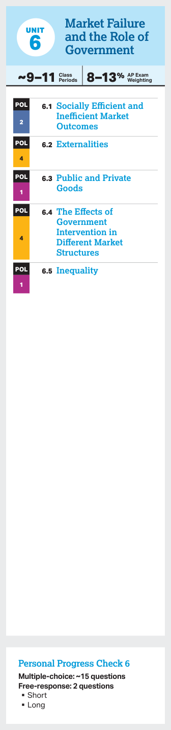
6.4 The Effects of Government Intervention in Different Market Structures** `[POL]`

6.4 The Effects of Government Intervention in Different Market Structures** [POL]

A policy that changes a price changes behavior: consumers alter quantity demanded, producers alter quantity supplied, and the resulting equilibrium may improve or reduce efficiency. The central question is not simply whether government intervenes, but whether the intervention corrects the incentive responsible for the market failure.

Learning Objective POL-4.A: Explain how government intervention affects outcomes in different market structures.
Essential Knowledge: POL-4.A.1–POL-4.A.7

One policy, different market outcomes

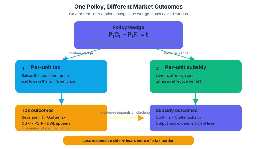
A per-unit tax creates a wedge between the price consumers pay and the net price firms receive. A subsidy creates the opposite wedge. The size of the resulting change depends partly on the price elasticities of demand and supply: the less responsive side of the market generally bears more of a tax burden.

For a per-unit tax of $t$, the relationship is:

$$P_C - P_F = t$$

where $P_C$ is the consumer price and $P_F$ is the firm’s net price. The tax usually reduces equilibrium quantity, consumer surplus, and producer surplus, while creating government revenue:

$$\text{Government revenue} = t \times Q_{\text{after tax}}$$

The lost surplus that is not transferred to the government is deadweight loss—the reduction in total economic surplus caused by mutually beneficial trades no longer occurring.

A per-unit subsidy reverses the direction of the wedge. It lowers the effective marginal cost of production or raises the effective marginal benefit of consumption, increasing equilibrium quantity. Government cost is:

$$\text{Government cost} = \text{per-unit subsidy} \times Q_{\text{after subsidy}}$$

Without a market failure, a subsidy can push output beyond the socially efficient quantity and create additional deadweight loss. With a positive externality, however, a subsidy may move output toward the socially optimal quantity.

Lump-sum policies versus per-unit policies

A lump-sum tax is a fixed payment that does not depend on the number of units produced or consumed. It changes fixed cost, but not marginal cost; therefore, it does not change the firm’s short-run profit-maximizing output rule, $MR = MC$. A lump-sum subsidy similarly changes fixed cost or fixed benefit without changing marginal cost or marginal benefit.

Misconception check: “Any tax reduces output.”
A per-unit tax changes the marginal incentive to produce or consume. A lump-sum tax does not. It may reduce profit, but it does not shift the firm’s marginal cost curve.

Price controls across market structures

A binding price ceiling or price floor does not have one universal effect across all markets. Its result depends on the market structure and on the elasticities of demand and supply.

In perfect competition, a binding price ceiling below equilibrium creates a shortage because quantity demanded exceeds quantity supplied. A binding price floor above equilibrium creates a surplus. In monopoly, the government must analyze the firm’s demand, marginal revenue, and marginal cost rather than treating the monopolist like a price-taking firm. In monopsony, a wage floor can sometimes increase both the wage and employment when it is set within the relevant range, because it limits the buyer’s wage-setting power.

Monopoly regulation: fair return versus marginal-cost pricing

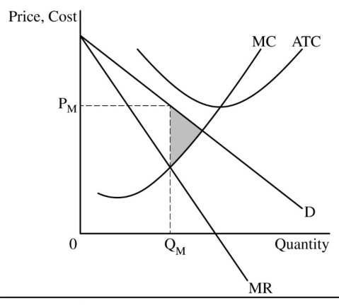
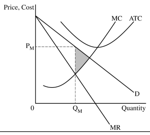
A monopolist chooses output where $MR = MC$, then charges the price found on the demand curve. Because the monopolist faces a downward-sloping demand curve, its marginal revenue lies below demand: selling one more unit requires lowering the price on all units, not merely on the additional unit.

The socially efficient quantity occurs where demand, interpreted as marginal benefit, intersects marginal cost:

$$MB = MC$$

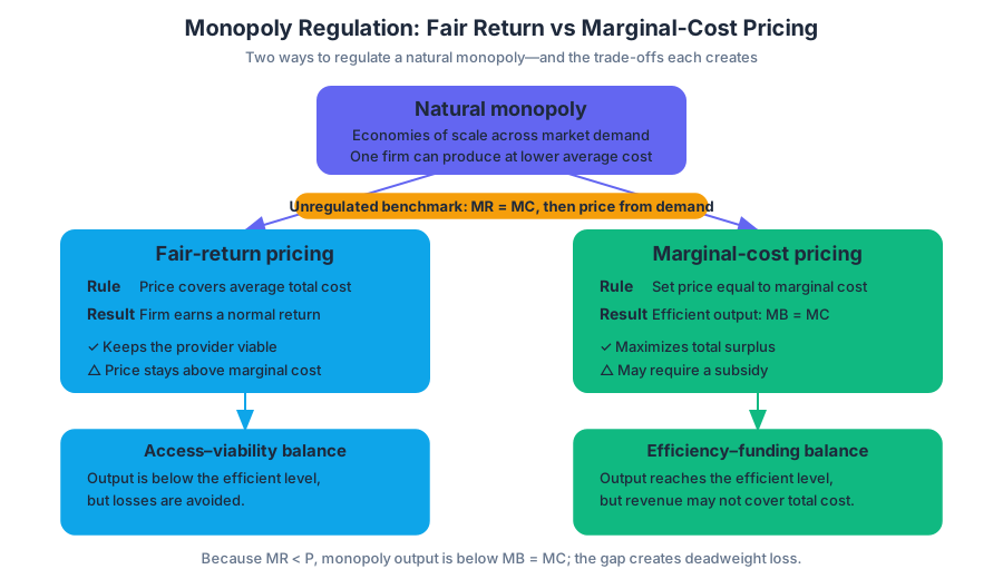
For a monopoly, this efficient quantity is greater than the profit-maximizing quantity because $MR < P$. The output gap creates deadweight loss, represented graphically by the area between the demand and marginal cost curves over the units not produced.

A natural monopoly has economies of scale across the entire range of market demand, so one firm can produce at a lower average total cost than several competing firms. Two common regulatory choices are:

Policy	Rule	Result
Fair-return regulation	$P = ATC$	The firm earns zero economic profit, but output may remain below the efficient quantity
Marginal-cost pricing	$P = MC$	Output is allocatively efficient, but price may fall below $ATC$

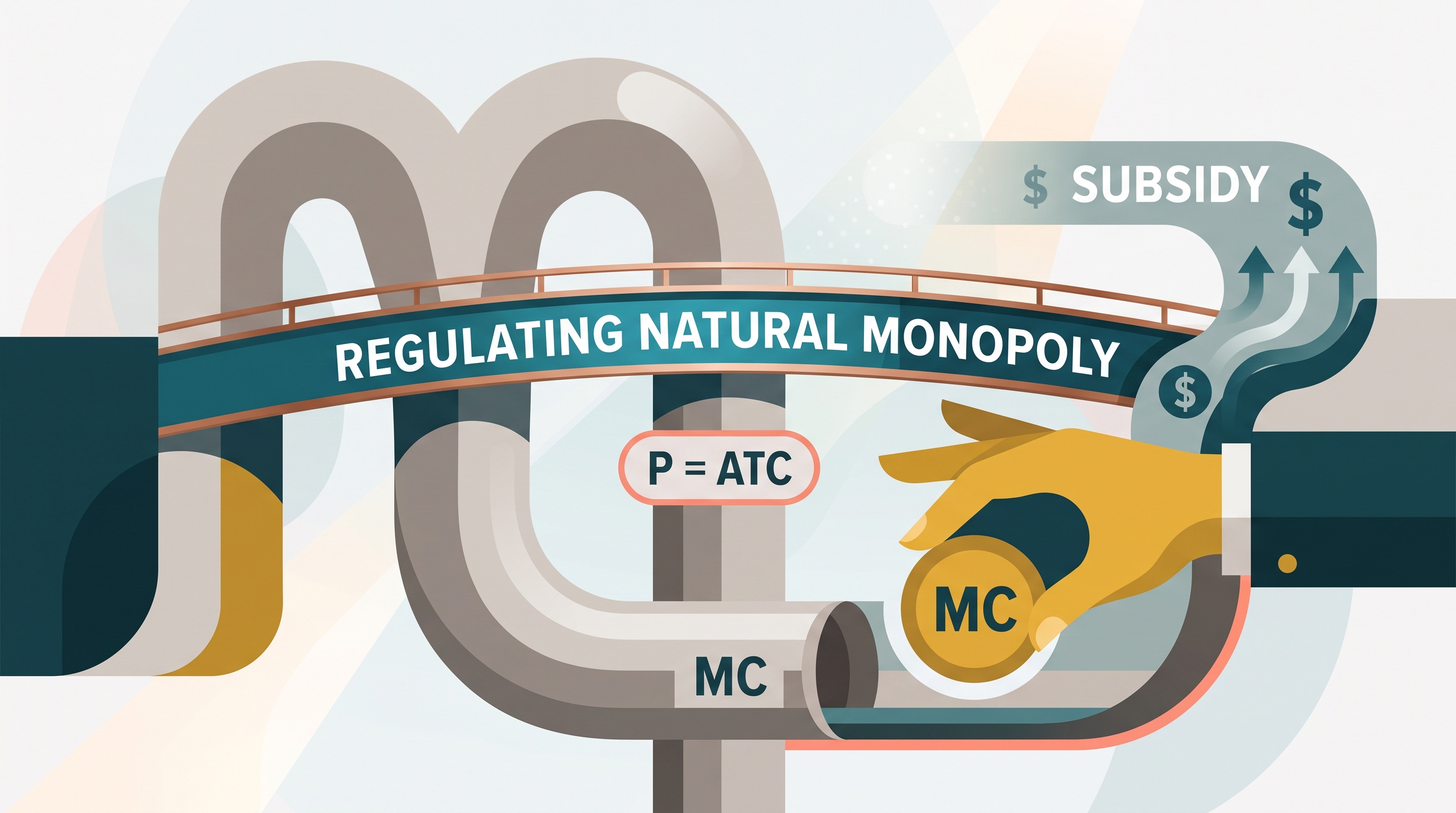
Fair-return regulation can leave allocative inefficiency because the regulated price may still exceed marginal cost. Marginal-cost pricing reaches the socially optimal quantity, but a natural monopoly may require a lump-sum subsidy to cover losses when $P = MC < ATC$. The subsidy supports operation without changing the marginal-cost incentive.

Correcting incentives and increasing competition

Government intervention increases efficiency when it addresses the incentive that caused the market failure. A tax equal to the marginal external cost can internalize a negative externality; a subsidy can encourage an activity with external benefits; price regulation can constrain monopoly power; and antitrust policy attempts to make markets more competitive through measures such as preventing anticompetitive mergers.

Key distinction: Government intervention is not automatically efficient. The relevant test is whether the policy moves production toward the socially optimal quantity while minimizing unintended distortions.

Retrieval check

A natural monopoly is currently regulated at $P = ATC$, but this price remains above $MC$. Is the outcome allocatively efficient? What regulation would reach the efficient quantity, and why might that policy require a lump-sum subsidy?