5.2 Changes in Factor Demand and Factor Supply** `[PRD]`

5.2 Changes in Factor Demand and Factor Supply** [PRD]

A firm hires an additional worker only when that worker adds enough revenue to justify the wage. In a perfectly competitive labor market, the market determines the wage, so the firm treats the wage as its marginal resource cost—the extra cost of hiring one more unit of a resource.

PRD-4.A Learning Objective: Explain the relationship between factors of production, firms, and factor prices, using graphs where appropriate, and calculate marginal revenue product (MRP) and marginal resource cost (MRC) from a graph or table.

The hiring decision: value the worker’s contribution

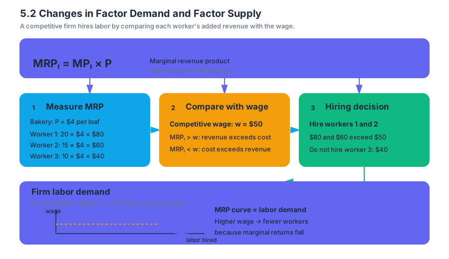
Marginal revenue product (MRP) is the additional revenue generated by employing one more unit of a factor. For labor, the usual calculation is:

$$ MRP_L = MP_L \times P $$

where $MP_L$ is the marginal product of labor—the additional output produced by one more worker—and $P$ is the market price of the firm’s output.

Suppose a bakery sells each loaf for $4. The first worker produces 20 additional loaves, the second produces 15 additional loaves, and the third produces 10 additional loaves.

Worker hired	$MP_L$	Output price $P$	$MRP_L = MP_L \times P$
1	20 loaves	$4	$80
2	15 loaves	$4	$60
3	10 loaves	$4	$40

If the competitive wage is $50 per worker, the bakery compares each worker’s MRP with the wage. The first and second workers add more revenue than they cost, so they are worth hiring. The third worker adds only $40 but costs $50, so the firm does not hire that worker.

$$ MRP_L > w \Rightarrow \text{hire the worker} $$

$$ MRP_L < w \Rightarrow \text{do not hire the worker} $$

In a perfectly competitive labor market, the individual firm is a wage taker. It cannot raise or lower the market wage by changing its own employment. Therefore:

$$ MRC_L = w $$

The firm’s labor-demand curve is its MRP curve: as the wage rises, the firm hires fewer workers whose MRP meets or exceeds that wage. This creates a downward-sloping quantity of labor demanded.

Why labor demand shifts

A change in the wage causes a movement along the firm’s labor-demand curve. A change in a determinant of MRP shifts the entire curve. Under PRD-4.B.1, the major determinants include the firm’s output price and worker productivity.

If bottled-water demand increases, the price of bottled water may rise. Because $MRP_L = MP_L \times P$, a higher output price raises the MRP of each worker. At every possible wage, the firm now wants to hire more labor: labor demand shifts right.

The same result occurs when worker productivity increases. Better training, improved tools, or a more efficient production process raises $MP_L$, increasing MRP at every wage. In contrast, a fall in the output price or worker productivity shifts labor demand left.

Misconception check: A higher wage does not shift labor demand right or left. It changes the quantity of labor demanded—a movement along the curve. Output price and productivity shift labor demand.

Why labor supply shifts

The market labor-supply curve shows how much labor workers are willing and able to offer at different wages. Holding other factors constant, quantity of labor supplied is positively related to the wage: a higher wage encourages more people to work or more hours of work.

Under PRD-4.B.2, labor-supply determinants include immigration, education, working conditions, age distribution, availability of alternative jobs, preferences for leisure, and cultural expectations. More immigration or expanded training may shift labor supply right. Safer working conditions, more attractive alternatives, or a stronger preference for leisure may reduce labor supplied and shift the curve left.

These shifts affect the equilibrium wage and employment in the labor market. For example, a decrease in the supply of workers shifts labor supply left, raising the equilibrium wage and reducing equilibrium employment, assuming labor demand remains unchanged.

Factor prices and income distribution

Factor markets distribute income among the owners of the factors of production: labor receives wages, capital receives interest, and land receives rent. The same reasoning applies beyond labor: firms compare the MRP of each input with its factor price and seek an allocation in which the last dollar spent on each input produces the same additional revenue.

The relevant AP skills are Skill 1.A: Define economic principles and models, when identifying MRP, MRC, and factor-market relationships; Skill 2.B: Explain economic outcomes, when connecting output prices or productivity to labor demand; Skill 3.A: Determine outcomes of specific economic situations, when predicting changes in wages and employment; Skill 3.B: Solve quantitative problems using economic concepts, when calculating $MRP_L$; and Skill 4.A: Draw and label graphs or visual representations plus Skill 4.B: Represent economic situations using graphs or visual representations, when showing curve shifts and new equilibrium outcomes.

Retrieval check

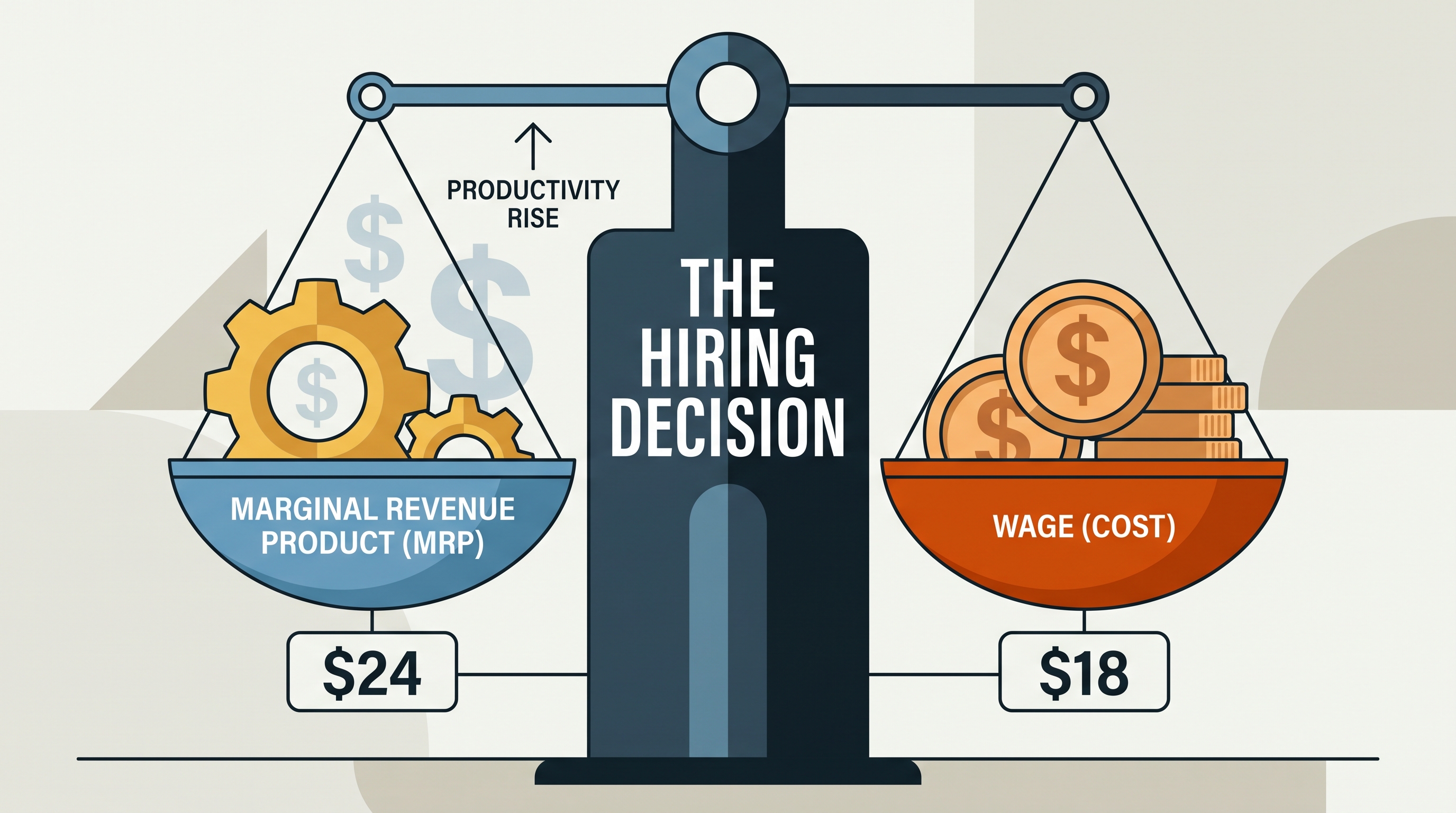
A firm pays a wage of $18. A worker’s marginal product is 6 units, and the output price is $4 per unit. Calculate MRP and decide whether the worker should be hired.

The answer is:

$$ MRP_L = 6 \times $4 = $24 $$

Because $$24 > $18$, the worker adds more revenue than cost and should be hired. If worker productivity rises, labor demand shifts right; if only the wage rises, the firm moves upward along its existing labor-demand curve.