2.3 Price Elasticity of Demand** `[MKT]`

2.3 Price Elasticity of Demand** [MKT]

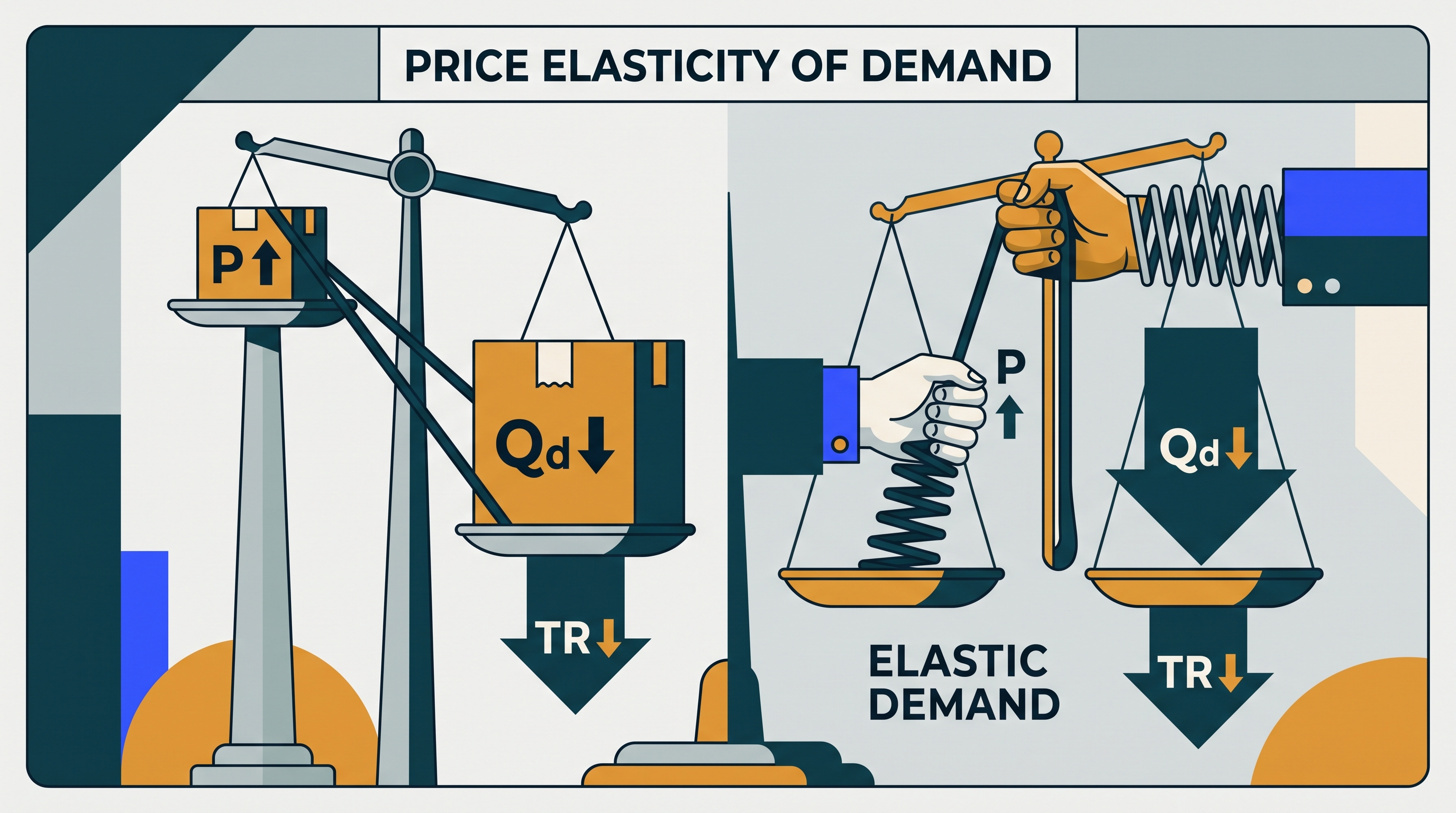
When the price of movie tickets rises, some people still attend, while others switch to streaming, wait for a discount, or skip the movie entirely. Price elasticity of demand measures how strongly quantity demanded responds to a change in a good’s own price.

From the law of demand to elasticity

The law of demand states that, holding other influences constant, a change in a good’s own price causes an opposite-direction change in quantity demanded. A higher price causes a movement upward along the existing demand curve and a lower quantity demanded; a lower price causes a movement downward along that curve and a higher quantity demanded. This is a movement along the demand curve, not a shift of the curve.

MKT-3.E.1: Elasticity measures the magnitude of percentage changes in quantity resulting from changes in own-price, income, or prices of related goods.

Price elasticity of demand, abbreviated PED, focuses specifically on responsiveness to the good’s own price:

$$ PED=\frac{%\Delta Q_d}{%\Delta P} $$

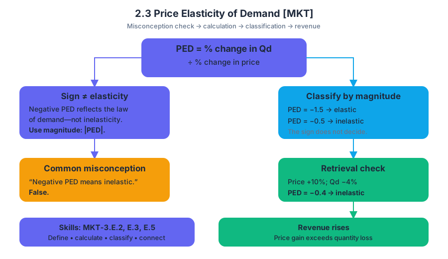
Here, $%\Delta Q_d$ is the percentage change in quantity demanded, and $%\Delta P$ is the percentage change in the good’s own price. Because price and quantity demanded generally move in opposite directions, PED is usually negative. Economists classify demand using the magnitude—the absolute value—of PED, so the negative sign does not determine whether demand is elastic or inelastic.

The benchmark of $1$

The number $1$ is the dividing line because it represents proportional responsiveness: a $1%$ change in price produces a $1%$ change in quantity demanded.

Demand classification	Magnitude of PED	Interpretation
Elastic	$	PED
Inelastic	$	PED
Unit elastic	$	PED

Worked example. A concert venue raises its ticket price from $$10$ to $$12$, while quantity demanded falls from $100$ tickets to $70$ tickets.

$$ %\Delta P=\frac{12-10}{10}=20% $$

$$ %\Delta Q_d=\frac{70-100}{100}=-30% $$

$$ PED=\frac{-30%}{20%}=-1.5 $$

Because $|PED|=1.5>1$, demand is elastic over this particular price change. Quantity demanded falls proportionally more than price rises.

A crucial graphing distinction is that slope is not elasticity. Slope compares changes in levels—such as dollars per ticket divided by tickets—whereas elasticity compares percentage changes. Elasticity can vary along a straight-line demand curve even though that curve has a constant slope.

What determines responsiveness?

The most important factor emphasized in MKT-3.E.4 is the availability of substitutes—alternative goods that satisfy a similar want. Demand for one brand of bottled water is often relatively elastic because consumers can switch to another brand. Demand for water itself may be more inelastic when no close alternative is available.

Consumers respond to price incentives, but their responses are constrained by income, time, and legal or regulatory frameworks. A small price increase may strongly affect a low-income household’s purchase decision. Given more time, consumers may find substitutes, change habits, or purchase durable equipment instead; immediately, they may have fewer options. Regulations can also limit which alternatives are legally available.

Total revenue: the practical payoff

Total revenue, or total expenditure from the consumer’s perspective, is:

$$ TR=P\times Q $$

The effect of a price change depends on elasticity because price and quantity move in opposite directions.

Demand is…	If price rises	If price falls
Elastic	Total revenue falls	Total revenue rises
Inelastic	Total revenue rises	Total revenue falls
Unit elastic	Total revenue is unchanged	Total revenue is unchanged

For the concert venue, revenue initially equals $$10\times100=$1{,}000$. After the price increase, revenue is $$12\times70=$840$. The price rose, but the elastic demand response caused quantity—and therefore total revenue—to fall enough to outweigh the higher price.

Misconception check and retrieval

Named misconception: “A negative PED means demand is inelastic.” False. The negative sign reflects the law of demand. Classification uses magnitude: $PED=-1.5$ is elastic, while $PED=-0.5$ is inelastic.

Retrieval check: If price rises by $10%$ and quantity demanded falls by $4%$, calculate PED, classify demand, and predict total revenue. The answer is $PED=-0.4$, so demand is inelastic; total revenue rises because the percentage increase in price exceeds the percentage decrease in quantity demanded. These calculations apply MKT-3.E.2, MKT-3.E.3, and MKT-3.E.5: define, calculate, classify, and connect elasticity to revenue.