From the free course AP Microeconomics on Lykke
3.7 Perfect Competition** `[PRD]`
Key concepts: Perfect competition · Nash equilibrium · Dominant strategies · Player payoffs and unilateral deviations · Strategic behavior in oligopoly and nonmarket settings · Economies of scale · Efficient scale · Long-run average total cost (LRATC) · Equilibrium behavior · Factor markets
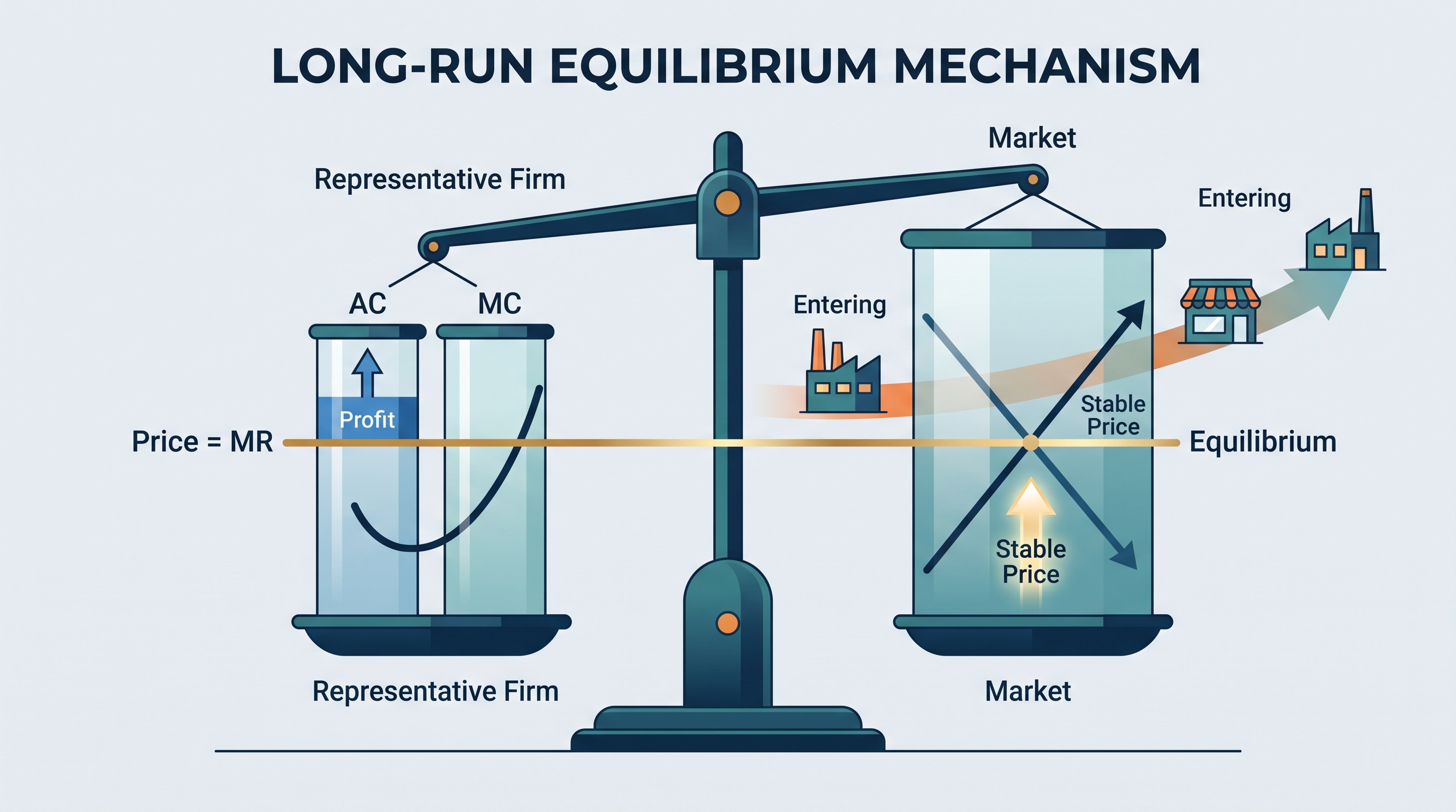
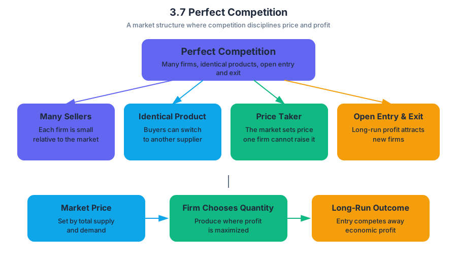
Perfect competition is a market structure in which many firms sell an identical product, individual firms are too small to influence the market price, and entry and exit are sufficiently open that long-run economic profit is competed away.
3.7 Perfect Competition** [PRD]
Perfect competition is a market structure in which many firms sell an identical product, individual firms are too small to influence the market price, and entry and exit are sufficiently open that long-run economic profit is competed away.
A wheat farmer can sell at the market price but cannot profitably charge more: buyers can purchase identical wheat from many other farms. The market determines the price; the individual firm chooses the quantity that makes its profit as large as possible.
The perfectly competitive firm: a price taker
The market demand and supply curves determine the equilibrium price, $P_M$. For the individual firm, that price becomes a horizontal demand curve because the firm can sell any feasible quantity at $P_M$, but essentially none at a higher price. Therefore:
$$ P = MR = AR $$
The firm selects its profit-maximizing output where marginal revenue equals marginal cost:
$$ MR = MC $$
Because a perfectly competitive firm is a price taker, $MR=P$. The firm therefore produces the quantity where:
$$ P = MC $$
This connects directly to the short-run decision rule established earlier: the firm produces at the quantity where $P=MC$ only if the price covers average variable cost. If price is below $AVC$, producing would not cover the costs that vary with output, so the firm shuts down in the short run.
Worked example: market equilibrium to firm equilibrium
Suppose the market price for a bushel of soybeans is $$14$. A soybean farm faces a horizontal firm demand curve at $$14$. If the farm’s marginal cost reaches $$14$ at $500$ bushels, then:
$$ P = MR = MC = $14 $$
The farm’s profit-maximizing quantity is therefore $500$ bushels. The farm does not choose the market quantity; it takes the market price and applies marginal analysis to choose its own output.
On an exam graph, label the market graph with downward-sloping demand, upward-sloping supply, equilibrium price $P_M$, and equilibrium quantity $Q_M$. On the firm graph, draw horizontal $d=MR$ at $P_M$, then locate the output where the rising $MC$ curve crosses that line. Missing the firm’s horizontal demand curve confuses a price-taking firm with a price-setting firm.
Perfect versus imperfect competition
Under perfect competition, the firm faces a perfectly elastic demand curve at the market price. Under imperfect competition, such as monopoly or oligopoly, a firm has some price-setting power and typically faces a downward-sloping demand curve. This distinction changes the relationship between price and marginal revenue:
$$ \text{Perfect competition: } P=MR $$
$$ \text{Imperfect competition: } P>MR $$
The difference matters for market outcomes. Oligopolists may attempt to coordinate or behave strategically, but they have difficulty achieving the monopoly outcome for reasons resembling the Prisoner’s Dilemma. Consequently, prices are generally higher and quantities lower with oligopoly or duopoly than with perfect competition.
Nash equilibrium and strategic behavior
A Nash equilibrium is a set of actions in which no player can increase their payoff by unilaterally changing actions, given the other players’ actions. It describes a stable strategic outcome—not necessarily the fairest, most efficient, or highest-total-payoff outcome.
PRD-3.C.6: A Nash equilibrium is a condition describing the set of actions in which no player can increase his or her payoff by unilaterally taking another action, given the other players’ actions.
Nash equilibrium applies to theoretical behavior in various oligopoly-market and nonmarket settings: competing firms choosing prices, businesses deciding whether to advertise, or individuals choosing actions when each person’s payoff depends partly on others’ choices. The central test is always unilateral deviation: hold everyone else’s action fixed and ask whether one player would gain by switching.
Consider this original two-firm payoff table. Each firm chooses High price or Low price; each ordered pair lists Firm A’s payoff first.
| Firm B: High price | Firm B: Low price | |
|---|---|---|
| Firm A: High price | $(8,8)$ | $(2,10)$ |
| Firm A: Low price | $(10,2)$ | $(4,4)$ |
For Firm A, Low price is a dominant strategy because it produces a higher payoff regardless of Firm B’s action: $10>8$ when B chooses High, and $4>2$ when B chooses Low. Firm B has the same dominant strategy. The Nash equilibrium is therefore $(\text{Low},\text{Low})$, with payoffs $(4,4)$: neither firm can improve by changing alone.
To calculate the incentive sufficient to alter a player’s dominant strategy, compare the payoff from following the dominant strategy with the best payoff from deviating, holding the other player’s action constant. If Firm B chooses Low, Firm A receives $4$ from Low and only $2$ from High. The deviation penalty is:
$$ $4-$2=$2 $$
Firm A would need at least a $$2$ additional incentive attached to High price to make deviation worthwhile.
PRD-3.C: Define key terms, strategies, and concepts relating to oligopolies and simple games; explain strategies and equilibria in theoretical oligopoly-market and nonmarket settings; and calculate the incentive sufficient to alter a player’s dominant strategy.
The course scope excludes games with more than two players or more than two actions per player, mixed-strategy equilibria, extensive-form games, and normal-form games exceeding two players or two actions per player.
Economies of scale and efficient scale
Economies of scale occur when long-run average total cost, $LRATC$, falls as output increases. The efficient scale is the output level that minimizes $LRATC$. At outputs beyond that point, $LRATC$ rises, indicating diseconomies of scale.
Suppose a furniture producer has total cost of $$80{,}000$ at $500$ chairs:
$$ LRATC=\frac{$80{,}000}{500}=$160\text{ per chair} $$
If producing $600$ chairs raises $LRATC$ to $$180$ per chair, the firm experiences diseconomies of scale over that range. Do not calculate the increase as $$280$ by adding the two per-unit costs; the correct comparison is:
$$ $180-$160=$20\text{ per chair} $$
In perfect competition, equilibrium analysis links firm decisions, market supply, and long-run entry or exit. In factor markets, the same marginal logic reappears: firms compare the additional revenue generated by an input with the additional cost of using it. Across both product and factor markets, equilibrium is a condition in which no decision-maker can improve by making a feasible unilateral adjustment.
Misconception check: A Nash equilibrium is not automatically a socially efficient outcome, and perfect competition is not the same as “every firm earns positive profit.” In long-run competitive equilibrium, entry and exit tend to eliminate economic profit, while the efficient scale concerns minimum $LRATC$, not maximum total output.
Retrieval check: A competitive firm faces $P=$12$ and chooses output where $MC=$12$. If another firm enters and market supply increases, what happens first to the market price, the firm’s horizontal demand curve, and the firm’s profit? Explain each change using price-taking and entry logic.
Source Materials
- AP Microeconomics Course and Exam Description
- AP Microeconomics Course and Exam Description Clarifications and Corrections
- AP Microeconomics Course Overview
- AP Microeconomics Course at a Glance
- AP Microeconomics Course at a Glance Poster
- AP Microeconomics
- AP Microeconomics
- AP Microeconomics Sample Syllabus 1