AP Practice 5

AP Practice 5

A numerical-analysis response earns more than a final number: it must expose the economic relationship that makes the number meaningful. In this practice, the central task is to use a market model to calculate equilibrium, consumer and producer surplus, and the efficiency loss created by a policy.

Exam task type: free-response numerical analysis, supported by interpretation and graphing. The current AP Microeconomics exam includes three free-response questions and assesses numerical analysis, economic reasoning, graphing, and written explanation. Treat the problem below as original and unofficial practice.

The market for reusable meal containers

A city’s market for reusable meal containers is described by the following equations, where $P$ is the price in dollars per container and $Q$ is the number of containers traded:

$$ Q_D = 120 - 2P $$

$$ Q_S = 20 + 2P $$

The city initially allows the market to operate without intervention. It then imposes a per-unit tax of $10$ on sellers.

Suggested timing: Spend about $12$ minutes. Reserve the final $2$ minutes to check algebra, units, graph labels, and whether each numerical answer is connected to the correct economic area.

Part A — Find the initial equilibrium

Set quantity demanded equal to quantity supplied:

$$ 120 - 2P = 20 + 2P $$

$$ 100 = 4P $$

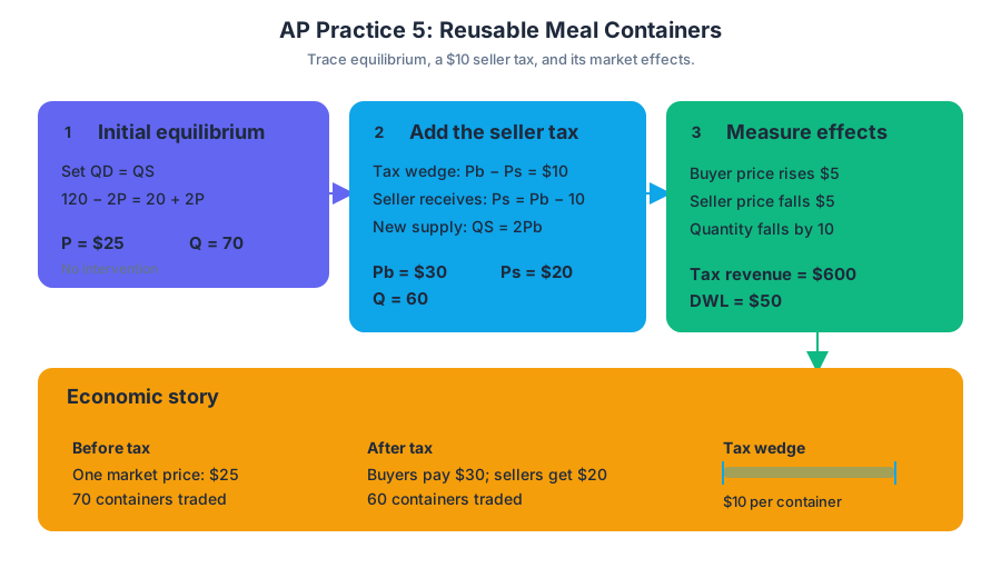
$$ P = 25 $$

Substitute $P=25$ into either equation:

$$ Q = 120 - 2(25) = 70 $$

The initial equilibrium is therefore a price of $$25$ and a quantity of $70$ containers. A complete numerical response should include both variables and their units, not merely the algebraic value.

Reward-worthy conclusion: The market equilibrium is $\left(P,Q\right)=\left($25,70\right)$.

Part B — Calculate the initial surplus

Rewrite each curve in inverse form to identify the intercepts. Demand is:

$$ Q_D=120-2P $$

At $Q=0$:

$$ 0=120-2P \Rightarrow P=60 $$

Supply is:

$$ Q_S=20+2P $$

At $Q=0$:

$$ 0=20+2P \Rightarrow P=-10 $$

Consumer surplus is the triangular area below the demand curve and above the equilibrium price:

$$ CS=\frac{1}{2}(70)(60-25)=$1{,}225 $$

Producer surplus is the area above the supply curve and below the equilibrium price. Because the supply curve crosses the price axis at $-$10$, the relevant height is:

$$ PS=\frac{1}{2}(70)(25-(-10))=$1{,}225 $$

Thus total surplus is:

$$ TS=CS+PS=$1{,}225+$1{,}225=$2{,}450 $$

Common error — treating a negative supply intercept as impossible: A negative vertical intercept does not mean the firm pays consumers in the actual market. It is an algebraic extension of the supply curve used to calculate the area. The surplus calculation remains valid within the model.

Part C — Analyze the $10$ per-unit tax

Let $P_B$ represent the price paid by buyers. Sellers receive the buyer price minus the tax, so their net price is $P_B-10$. The after-tax supply relationship is therefore:

$$ Q_S=20+2(P_B-10) $$

$$ Q_S=2P_B $$

Set this equal to demand:

$$ 120-2P_B=2P_B $$

$$ P_B=30 $$

The quantity traded is:

$$ Q=120-2(30)=60 $$

Sellers receive:

$$ P_S=P_B-10=$20 $$

The tax raises the buyer price from $$25$ to $$30$, lowers the seller price from $$25$ to $$20$, and reduces quantity from $70$ to $60$. These three changes should appear together in a strong response because they demonstrate the tax wedge and the resulting contraction in trade.

Tax revenue equals the tax per unit multiplied by the quantity sold:

$$ TR=($10)(60)=$600 $$

After-tax consumer surplus is:

$$ CS=\frac{1}{2}(60)(60-30)=$900 $$

After-tax producer surplus is:

$$ PS=\frac{1}{2}(60)(20-(-10))=$900 $$

Total surplus including government revenue is:

$$ TS=$900+$900+$600=$2{,}400 $$

Therefore, deadweight loss is:

$$ DWL=$2{,}450-$2{,}400=$50 $$

What an examiner rewards

A high-quality numerical-analysis response does the following:

• identifies the initial equilibrium as $P=$25$ and $Q=70$;
• calculates the supply and demand intercepts before finding surplus;
• distinguishes the buyer price $P_B=$30$ from the seller price $P_S=$20$;
• calculates tax revenue using the post-tax quantity;
• includes consumer surplus, producer surplus, and government revenue in total surplus;
• identifies the deadweight loss as $$50$ and connects it to the reduction in mutually beneficial trades.

Misconception check: The tax does not eliminate all surplus, and the government’s tax revenue is not itself deadweight loss. Tax revenue is a transfer from buyers and sellers to the government; deadweight loss is the surplus from trades that no longer occur.

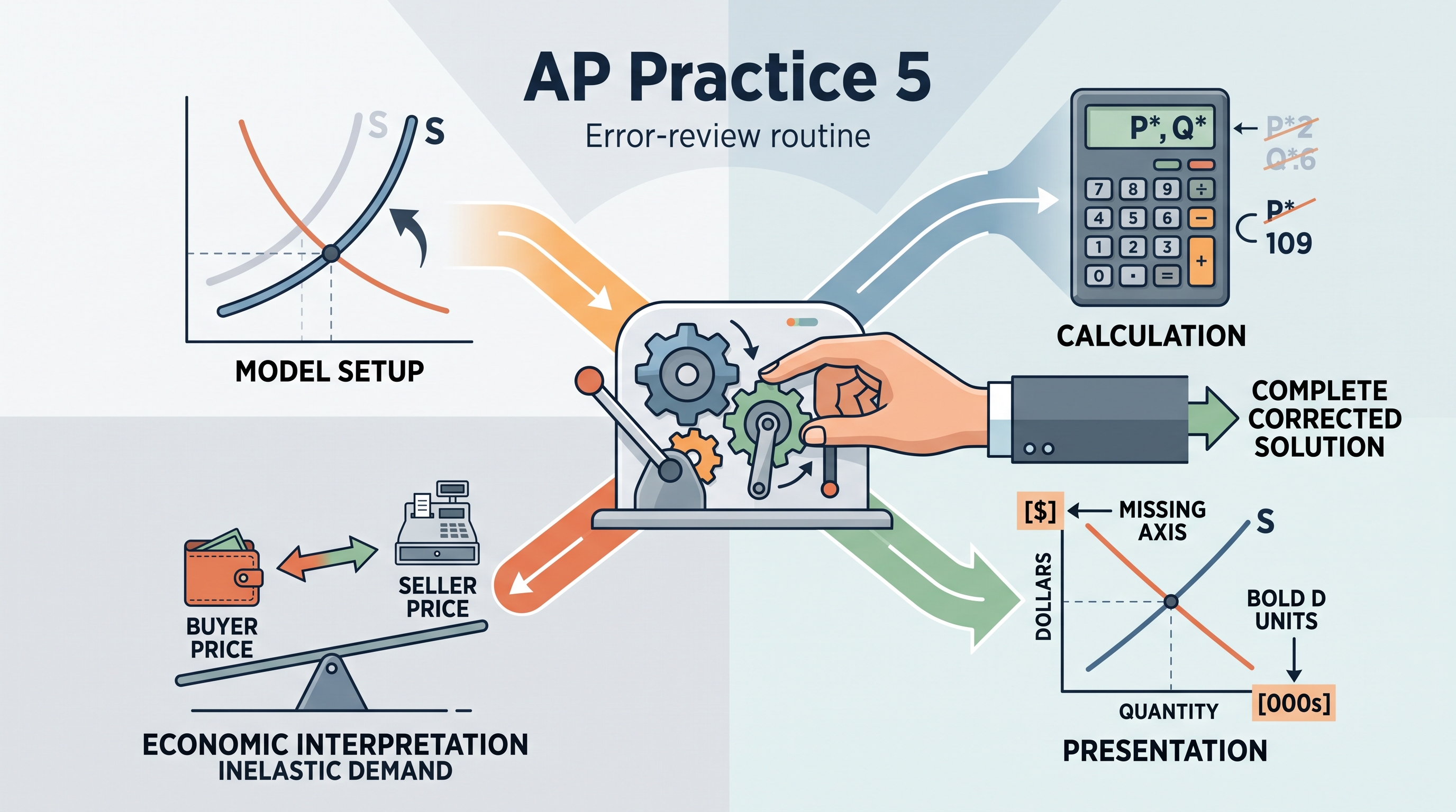
Error-review routine

After completing the problem, label your error as one of four types: model setup—such as shifting the wrong curve; calculation—such as solving the equilibrium incorrectly; economic interpretation—such as confusing buyer and seller prices; or presentation—such as omitting units or graph labels. Redo only the failed step, then explain in one sentence why the corrected step works.

Retrieval check: If demand were more inelastic than supply, which side would bear more of the $10$ tax? The less elastic side would bear more of the tax burden because it changes quantity less in response to the price change.