From the free course AP Microeconomics on Lykke
2.7 Market Disequilibrium and Changes in Equilibrium** `[MKT]`
Key concepts: Market equilibrium · Market disequilibrium · Shortage · Surplus · Shifts in supply and demand · Changes in equilibrium price and quantity · Consumer surplus · Producer surplus · Price elasticity of demand and supply · Marginal benefit and marginal cost
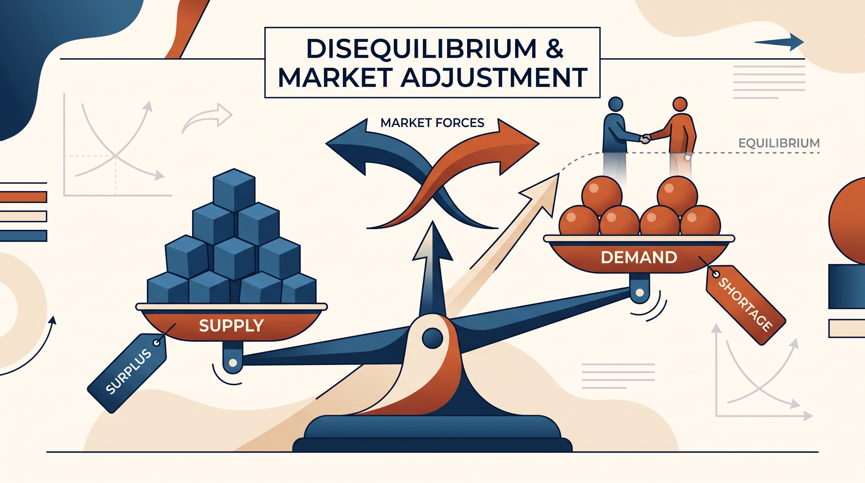
A market does not remain stuck when buyers and sellers disagree: price signals push quantity demanded and quantity supplied toward equality. If oranges are priced below the market-clearing level, for example, shoppers want more oranges than sellers offer.
2.7 Market Disequilibrium and Changes in Equilibrium** [MKT]
A market does not remain stuck when buyers and sellers disagree: price signals push quantity demanded and quantity supplied toward equality. If oranges are priced below the market-clearing level, for example, shoppers want more oranges than sellers offer. The result is a shortage, not a mysterious disappearance of oranges.
Equilibrium versus disequilibrium
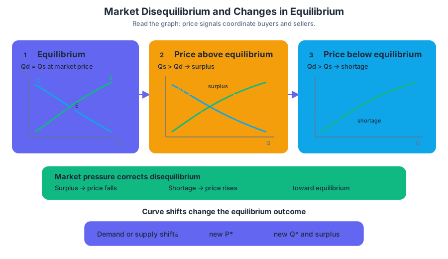
Market equilibrium occurs where quantity demanded equals quantity supplied, written as $Q_d = Q_s$. The corresponding price and quantity are the equilibrium price $P^$ and equilibrium quantity $Q^$.
Market equilibrium: the price and quantity at which the amount buyers want to purchase exactly equals the amount sellers want to sell.
At a price below $P^$, $Q_d > Q_s$: a shortage exists. At a price above $P^$, $Q_s > Q_d$: a surplus exists. Competitive market forces tend to remove these imbalances because shortages create upward pressure on price, while surpluses create downward pressure.
| Price condition | Buyer–seller relationship | Disequilibrium | Pressure on price |
|---|---|---|---|
| Below $P^*$ | $Q_d > Q_s$ | Shortage | Upward |
| At $P^*$ | $Q_d = Q_s$ | Equilibrium | No disequilibrium pressure |
| Above $P^*$ | $Q_s > Q_d$ | Surplus | Downward |
Worked example: oranges below equilibrium
Suppose the equilibrium price of oranges is $$2$ per bag. At that price, consumers demand and producers supply $500$ bags. If the price is held at $$1$, consumers may demand $700$ bags while producers supply only $300$ bags:
$$\text{Shortage} = Q_d - Q_s = 700 - 300 = 400\text{ bags}.$$
The precise statement is the quantity demanded of oranges is greater than the quantity supplied. It is not necessarily correct to say that the quantity purchased is greater than the quantity sold: in an actual shortage, the quantity successfully purchased and sold is limited by the smaller available amount, $300$ bags.
Misconception check — “A low price means everyone gets more.”
A lower price increases the quantity demanded, but it can reduce the quantity supplied. Without enough units available, some willing buyers cannot complete a purchase.
Changes in equilibrium: shifts, not movements
A change in an underlying market condition shifts an entire curve and creates a new equilibrium. A change in the good’s own price causes movement along a curve; it does not shift the curve. After a shift, compare the original and new equilibrium points to determine the changes in price, quantity, consumer surplus, and producer surplus.
For example, an increase in labor supply shifts the labor-supply curve rightward from $S_L$ to $S_L'$. Holding labor demand constant, the new equilibrium has a lower equilibrium wage and greater equilibrium employment:
$$ S_L \rightarrow S_L' \quad \Longrightarrow \quad w^* \downarrow,\quad L^* \uparrow. $$
This might occur when more workers become qualified for a job or when immigration expands the available workforce. The graph must show a vertical axis labeled wage, a horizontal axis labeled quantity of labor or employment, both supply curves, the demand curve, and the old and new equilibrium points.
Surplus after a market change
Consumer surplus is the area below the demand curve and above the market price for units purchased. Producer surplus is the area above the supply curve and below the market price for units sold. When a shock changes equilibrium, calculate the new areas from the appropriately labeled graph or table, then compare them with the original areas.
For a linear demand or supply curve, a triangular surplus is calculated as
$$\text{Triangle area}=\frac{1}{2}(\text{base})(\text{height}).$$
Suppose a market initially has price $$10$ and quantity $100$. If demand and supply shift so that the new equilibrium is price $$12$ and quantity $80$, consumers generally face a higher price and fewer purchases, so consumer surplus falls. Producers may gain or lose depending on the particular shift: the higher price helps sellers, but the reduction in units sold hurts them. The graph—not the price change alone—determines the exact change in producer surplus.
Elasticity matters: the direction of a change may be predictable, but its size depends partly on the price elasticities of demand and supply. A relatively inelastic curve produces a larger price response and a smaller quantity response than a relatively elastic curve when the same market shock occurs.
Efficient activity and marginal analysis
Market equilibrium is not the only setting in which marginal reasoning identifies an optimum. For any activity, the optimal level occurs where marginal benefit equals marginal cost:
$$MB = MC.$$
If a person evaluates study time, pollution reduction, or another activity, choosing $S_1$ hours when $MB > MC$ means under-investing: another hour creates more benefit than cost. Choosing $S_3$ hours when $MC > MB$ means over-investing. The optimal choice is $S_2$, where the two curves intersect.
AP reasoning and retrieval check
This topic activates Skill Category 1: Principles and Models, by identifying equilibrium, shortage, surplus, and surplus areas; Skill Category 2: Interpretation, by explaining what a graph or table implies in a specific market; Skill Category 3: Manipulation, by predicting the effects of curve shifts and calculating changed outcomes; and Skill Category 4: Graphing and Visuals, by drawing labeled axes, curves, equilibrium points, and directional changes. These skills connect directly to MKT-4.B.1, which emphasizes market forces correcting shortages and surpluses, and MKT-4.B.2, which links curve shifts to changes in price, quantity, and economic surplus.
Retrieval check: If a market price is above equilibrium, which relationship must be true—$Q_d > Q_s$ or $Q_s > Q_d$—and what direction will market pressure push the price? Explain in one sentence.
Source Materials
- AP Microeconomics Course and Exam Description
- AP Microeconomics Course and Exam Description Clarifications and Corrections
- AP Microeconomics Course Overview
- AP Microeconomics Course at a Glance
- AP Microeconomics Course at a Glance Poster
- AP Microeconomics
- AP Microeconomics
- AP Microeconomics Sample Syllabus 1