From the free course AP Microeconomics on Lykke
2.4 Price Elasticity of Supply** `[MKT]`
Key concepts: Price elasticity of supply · Responsiveness of quantity supplied to changes in price · Percentage changes in quantity supplied and price · Elastic supply · Inelastic supply · Unit elastic supply · Movement along a supply curve · Supply-curve shifts · Determinants of supply · Market supply as the summation of individual supply curves
Price elasticity of supply (PES) measures how strongly producers respond to a change in the good’s own price. If a small price increase causes sellers to expand production substantially, supply is elastic; if production changes only slightly, supply is inelastic.
2.4 Price Elasticity of Supply** [MKT]
Price elasticity of supply (PES) measures how strongly producers respond to a change in the good’s own price. If a small price increase causes sellers to expand production substantially, supply is elastic; if production changes only slightly, supply is inelastic.
MKT-3.D — Price elasticity of supply: PES is the percentage change in quantity supplied divided by the percentage change in price.
The formula is
$$ \text{PES}=\frac{%\Delta Q_s}{%\Delta P} $$
where $%\Delta Q_s$ is the percentage change in quantity supplied and $%\Delta P$ is the percentage change in price. Because price and quantity supplied usually move in the same direction, PES is normally positive. Classification depends on its magnitude.
| PES value | Type of supply | Meaning |
|---|---|---|
| $\text{PES}>1$ | Elastic supply | Quantity supplied changes by a larger percentage than price. |
| $\text{PES}<1$ | Inelastic supply | Quantity supplied changes by a smaller percentage than price. |
| $\text{PES}=1$ | Unit elastic supply | Quantity supplied and price change by the same percentage. |
Own-price changes: movement along supply
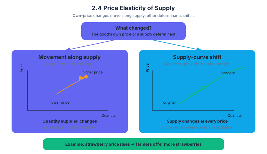
A change in a good’s own price does not shift the supply curve. Instead, it causes a movement along the existing supply curve and changes quantity supplied. For example, if the price of fresh strawberries rises, farmers move upward along their supply curve and offer more strawberries for sale.
The distinction is visual and causal:
A supply-curve shift has a different cause. Changes in determinants of supply—such as input availability or input prices—shift the entire curve. A cheaper fertilizer input can increase supply, shifting the supply curve rightward; a fertilizer shortage can decrease supply, shifting it leftward. These changes alter supply at every possible price rather than merely changing the quantity supplied at one price.
Worked example: classifying supply responsiveness
A bakery sells $100$ loaves per day when the price is $$2$ per loaf. When the price rises to $$2.20$, it increases daily production to $120$ loaves. Suppose the percentage changes are calculated relative to the original values:
$$ %\Delta Q_s=\frac{120-100}{100}=0.20=20% $$
$$ %\Delta P=\frac{2.20-2.00}{2.00}=0.10=10% $$
Therefore,
$$ \text{PES}=\frac{20%}{10%}=2 $$
Because $\text{PES}=2>1$, the bakery’s supply is elastic with respect to price. The bakery can respond strongly because it has available ovens, workers, and ingredients. If those inputs were difficult to obtain quickly, the same price increase might produce only a small increase in output, creating an inelastic supply response.
What determines PES?
Price elasticity of supply depends especially on the availability and price of inputs. Producers can respond more easily when labor, raw materials, equipment, or other inputs are readily available. Supply tends to be less responsive when inputs are scarce, expensive, or difficult to adjust in the relevant time period.
For example, a restaurant may expand meal production fairly quickly if it has unused kitchen capacity and can hire additional workers. A farmer cannot immediately create more mature crops after a sudden price increase, so agricultural supply may be relatively inelastic in the short run. The market’s PES reflects the combined responsiveness of all sellers in that market.
Misconception check
Misconception: “A higher price shifts supply to the right.”
Correction: A higher own price causes an upward movement along the supply curve and an increase in quantity supplied. A rightward shift in supply requires a change in a determinant such as input availability or input prices.
Another common error is treating “elastic” as synonymous with “large.” Elasticity is not the absolute amount produced; it is a ratio of percentage changes. A large producer can have inelastic supply, while a small producer can have elastic supply.
Retrieval check
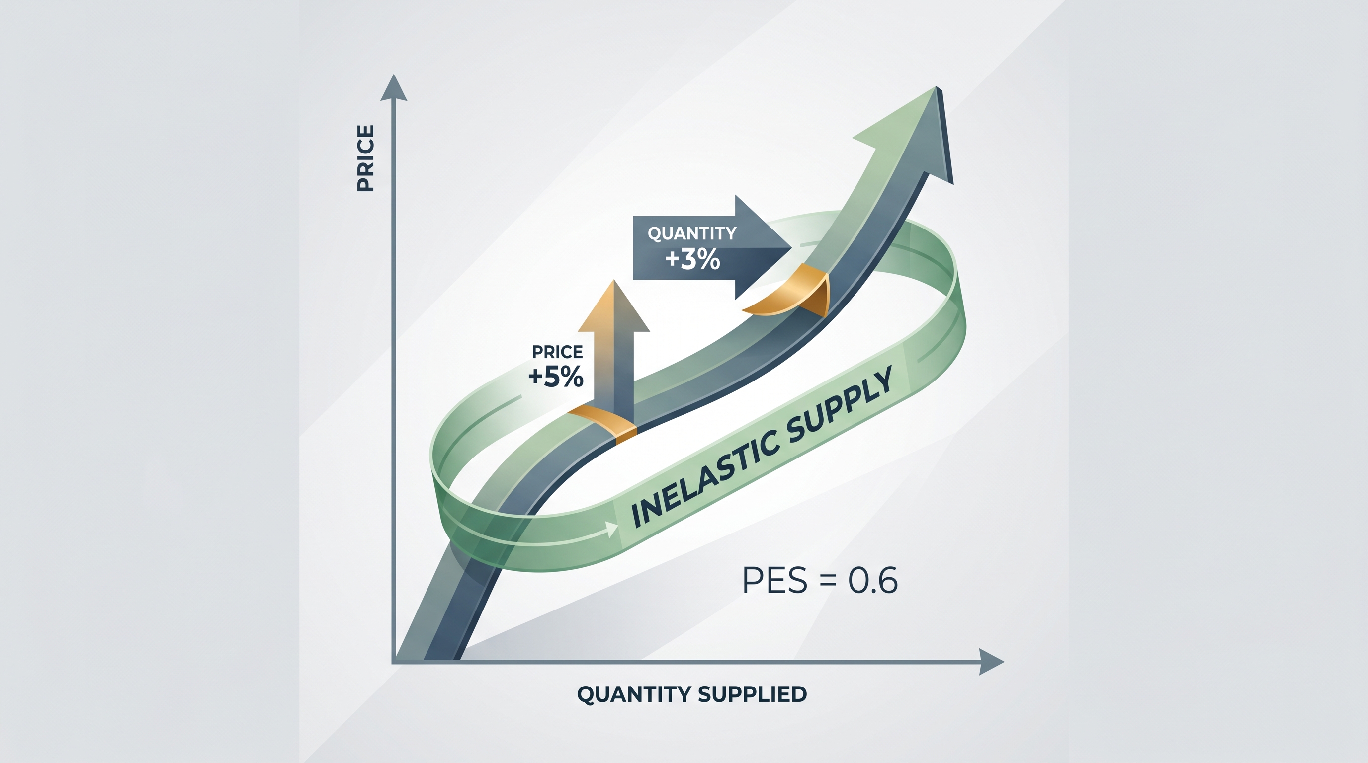
A price rises by $5%$, and quantity supplied rises by $3%$. Calculate and classify PES.
$$ \text{PES}=\frac{3%}{5%}=0.6 $$
Supply is inelastic because $\text{PES}<1$. Ask one final diagnostic question: did the price change move the producer along the supply curve, or did an input-related change shift the entire curve?
Source Materials
- AP Microeconomics Course and Exam Description
- AP Microeconomics Course and Exam Description Clarifications and Corrections
- AP Microeconomics Course Overview
- AP Microeconomics Course at a Glance
- AP Microeconomics Course at a Glance Poster
- AP Microeconomics
- AP Microeconomics
- AP Microeconomics Sample Syllabus 1
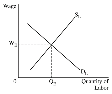
- (d)(ii) The graph from part (d)(i) must show a rightward shift in the labor supply curve, resulting in a lower equilibrium wage rate, labeled W2, and a higher equilibrium quantity of labor, labeled Q2
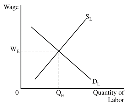
- (d)(ii) The graph from part (d)(i) must show a rightward shift in the labor supply curve, resulting in a lower equilibrium wage rate, labeled W2, and a higher equilibrium quantity of labor, labeled Q2
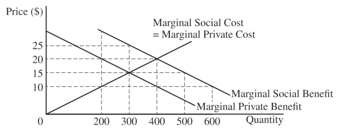
- (a) Identify the market equilibrium price and quantity.