3.3 Long-Run Production Costs** `[PRD]`

3.3 Long-Run Production Costs** [PRD]

A firm’s long run is the planning period in which every input can be changed. A bakery can expand its oven capacity, move to a larger building, hire more workers, or adopt new equipment; no input remains permanently fixed. Therefore, in the long run, all costs are variable. [PRD-1.A.9]

The long-run average total cost curve

Average total cost is total cost per unit of output:

$$ ATC=\frac{TC}{Q} $$

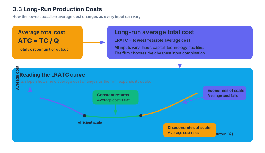
In the long run, long-run average total cost—abbreviated LRATC—shows the lowest possible average cost of producing each output level when all inputs are variable. For each quantity, the firm chooses the combination of labor, capital, technology, and facilities that produces that quantity as cheaply as possible.

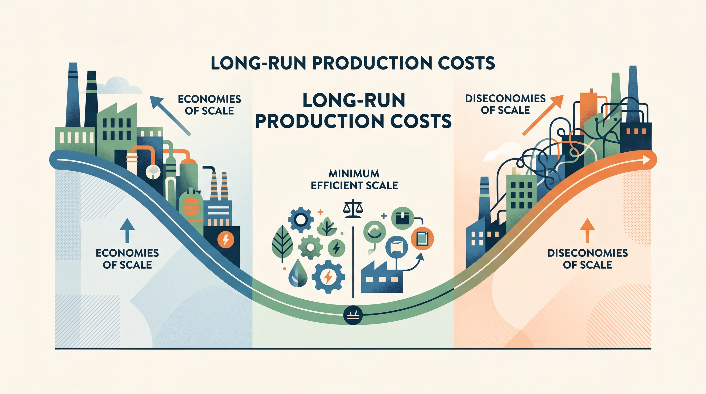
The LRATC curve is often broad and U-shaped. Its slope describes how average cost changes as the firm expands its scale of production, not merely how many units it produces in an unchanged facility.

LRATC segment	What happens as output rises?	Scale relationship
Downward-sloping	Average cost falls	Economies of scale
Flat	Average cost remains constant	Constant returns to scale
Upward-sloping	Average cost rises	Diseconomies of scale

[PRD-1.A.11]

Economies of scale

Economies of scale occur on the downward-sloping portion of the LRATC curve: expanding production lowers average cost. A larger firm may spread setup or management costs across more units, use specialized machinery, or divide production into focused tasks. Specialization and division of labor can reduce marginal costs by allowing workers to become faster and more productive at particular tasks [PRD-1.A.7].

Constant returns to scale

Constant returns to scale occur on the flat portion of LRATC. When all inputs increase proportionally, output rises proportionally and average cost does not change. If doubling every input doubles output, the firm experiences constant returns to scale. This region is also called the firm’s efficient scale when it represents the lowest attainable average cost.

Diseconomies of scale

Diseconomies of scale occur on the upward-sloping portion of LRATC: expanding further raises average cost. A very large organization may face communication delays, layers of management, coordination problems, or difficulty monitoring workers. Growth is no longer producing efficiency; it is producing complexity.

Returns to scale: the input-output relationship

Returns to scale describe how output responds when all inputs change together [PRD-1.A.10]. Increasing returns to scale mean output increases by a larger percentage than inputs. Constant returns to scale mean output increases by the same percentage. Decreasing returns to scale mean output increases by a smaller percentage.

For example, suppose a furniture firm doubles its labor, factory space, and machinery:

• If output rises from $1{,}000$ desks to $2{,}400$ desks, the firm has increasing returns to scale.
• If output rises to exactly $2{,}000$ desks, it has constant returns to scale.
• If output rises only to $1{,}600$ desks, it has decreasing returns to scale.

The terms “increasing” and “decreasing” describe the response of output to proportional input changes. On the LRATC graph, they usually correspond to economies and diseconomies of scale, respectively.

Connecting productivity and costs

The production relationship explains why cost curves change shape. In the short run, diminishing marginal returns occur when an additional variable input is combined with fixed inputs. As the marginal product of that input falls, producing another unit requires more of it, so marginal cost rises [PRD-1.A.6]. This is why a production function with diminishing marginal returns leads to an upward-sloping marginal cost curve.

Cost curves can also shift when input prices or productivity change [PRD-1.A.8]. A higher wage, more expensive electricity, or costlier raw materials shifts relevant cost curves upward. Better technology, improved worker productivity, or more effective specialization shifts them downward. A change in the firm’s output causes movement along a curve; a change in input costs or productivity shifts the curve itself.

Worked example: choosing scale

A meal-delivery company compares its lowest possible average costs at different production levels:

$$ \begin{aligned} Q=100 &: \quad LRATC=$12\ Q=200 &: \quad LRATC=$9\ Q=300 &: \quad LRATC=$9\ Q=400 &: \quad LRATC=$11 \end{aligned} $$

From $Q=100$ to $Q=200$, LRATC falls, so the firm experiences economies of scale. Between $Q=200$ and $Q=300$, LRATC is constant, indicating constant returns to scale. Beyond $Q=300$, LRATC rises, indicating diseconomies of scale. The minimum efficient scale begins where the firm reaches its lowest sustainable LRATC—here, at approximately $Q=200$.

Minimum efficient scale matters beyond the individual firm: if efficient production requires a very large output, only a few firms may be able to achieve low costs. That condition can contribute to a concentrated market and influence market structure [PRD-1.A.12].

Misconception check

Misconception: “Economies of scale mean the firm is earning a profit.” Economies of scale describe a cost pattern—average cost falls as output rises. Profit requires comparing revenue with total cost. A firm can have falling LRATC and still earn a loss if its price or revenue is sufficiently low.

AP skills and retrieval check

This topic activates Skill 1.A, “Define economic principles and models,” when identifying LRATC, returns to scale, and minimum efficient scale; Skill 1.B, “Explain economic principles and models,” when connecting scale to cost; Skill 3.B, “Calculate economic outcomes,” when computing average cost; and Skill 4.A, “Create representations,” and Skill 4.B, “Represent economic situations using graphs,” when labeling the LRATC curve and its three regions. The learning objective is PRD-1.A: define, explain, and calculate production and cost relationships.

Retrieval check: If a firm doubles every input but output increases by only $50%$, what type of returns to scale does it have, and which portion of the LRATC curve normally represents that outcome? Answer: decreasing returns to scale and the upward-sloping, diseconomies-of-scale portion.