5.3 Profit-Maximizing Behavior in Perfectly Competitive Factor Markets** `[PRD]`

5.3 Profit-Maximizing Behavior in Perfectly Competitive Factor Markets** [PRD]

A perfectly competitive firm does not choose workers by asking, “Can we afford another employee?” It asks a sharper question: Will the additional revenue generated by this worker exceed the worker’s cost? In a perfectly competitive factor market, the answer is found by comparing the worker’s marginal revenue product of labor with the market wage.

PRD-4: Factor prices provide incentives and convey information to firms and factors of production.

The firm as a price taker in the labor market

A factor market is a market for an input used to produce goods or services, such as labor, land, capital, or entrepreneurship. The factor price is the price paid for that input; for labor, it is the wage.

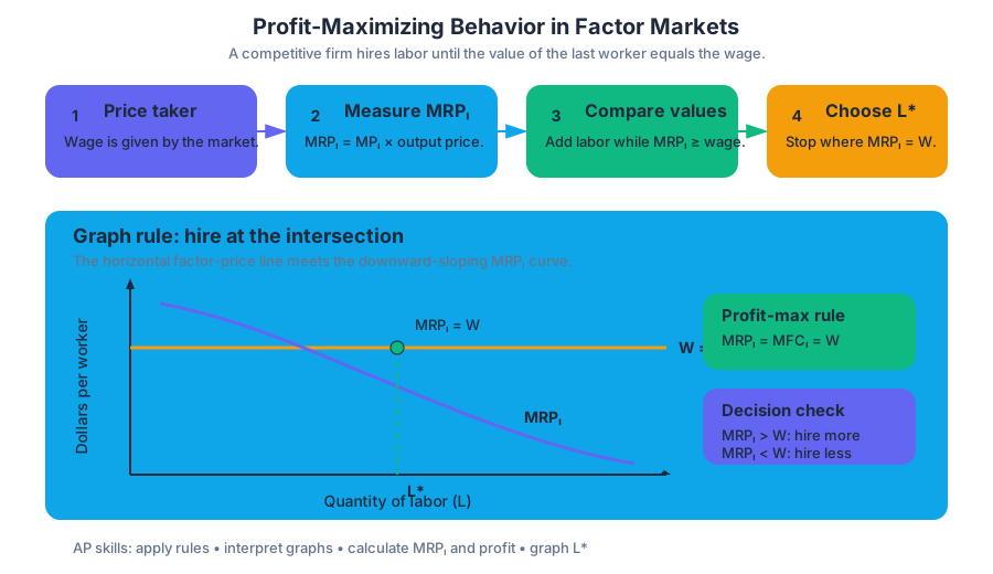
In a perfectly competitive labor market, many firms demand labor and many workers supply it. The market determines the wage, so one individual firm is too small to influence that wage. The firm is therefore a price taker: it can hire each additional worker at the same market wage.

This does not require the firm to be a perfect competitor in its output market. A firm might sell a differentiated product and possess some output-market power while still hiring workers in a competitive labor market. The relevant question is whether the firm can influence the wage, not whether it can influence the price of its final product.

For a price-taking firm, the marginal factor cost of labor, or $MFC_L$, equals the wage:

$$MFC_L = w$$

Because the firm can hire another worker without raising the wage paid to existing workers, its labor-supply curve is horizontal at the market wage. The firm compares this constant factor cost with the extra revenue produced by each worker.

Marginal revenue product and the hiring rule

The marginal revenue product of labor, written $MRP_L$, is the additional revenue created by hiring one more unit of labor. It combines two ideas: the additional output produced by the worker and the revenue earned from that output.

$$MRP_L = MP_L \times MR$$

Here, $MP_L$ is the worker’s marginal product—the additional output from one more worker—and $MR$ is the firm’s marginal revenue from selling one more unit of output. If the firm sells its output in a perfectly competitive product market, $MR=P$, so:

$$MRP_L = MP_L \times P$$

The profit-maximizing hiring rule is:

$$MRP_L = MFC_L$$

Since $MFC_L=w$ for a competitive factor market, the firm hires labor until:

$$MRP_L = w$$

The firm should continue hiring while $MRP_L>w$, because the worker adds more revenue than cost. It should not hire a worker when $MRP_L<w$, because that worker adds more cost than revenue.

Worked example: hiring labor one worker at a time

Suppose a bakery sells each additional box of pastries for $20. Its workers have the following marginal products:

Worker	$MP_L$	$MRP_L = MP_L \times MR$	Wage
1	$10$ boxes	$10 \times $20 = $200$	$$140$
2	$8$ boxes	$8 \times $20 = $160$	$$140$
3	$6$ boxes	$6 \times $20 = $120$	$$140$
4	$4$ boxes	$4 \times $20 = $80$	$$140$

The first two workers should be hired because each generates more revenue than the $140$ wage. The third worker should not be hired: $MRP_L=$120$ is less than the wage. Thus, the profit-maximizing employment level is two workers, where the last worker hired has $MRP_L \geq w$ and the next worker has $MRP_L<w$.

Why factor prices promote efficiency

Factor prices do more than determine who gets paid. They communicate information about the opportunity cost of using a resource and provide incentives to move resources toward valuable uses. A high wage signals that labor is relatively valuable in that use; a low wage makes it less costly for firms to employ labor there.

Under perfect competition and standard assumptions, factors flow toward their highest-valued uses because each firm hires labor until:

$$MRP_L = w$$

The wage is the same market price faced by competing firms. Therefore, labor continues moving toward a use whenever its marginal revenue product there exceeds the wage, and it stops moving when the marginal revenue product equals the wage. Across competing uses, this pushes marginal benefit toward equality with marginal cost: the additional value created by the last worker is equal to the opportunity cost of employing that worker. Mutually beneficial gains from reallocating labor are exhausted, producing an efficient allocation.

This connection parallels the product-market condition in perfect competition. Firms produce where $MR=MC$; because $MR=P$, they produce where $P=MC$. In factor markets, firms hire where $MRP_L=MFC_L$; because $MFC_L=w$, they hire where $MRP_L=w$. These price-taking conditions connect output, input use, and efficiency.

Profit, loss, and the exam graph

Economic profit or loss can be calculated from a graph or table:

$$\text{Economic profit} = TR - TC$$

It can also be expressed as:

$$\text{Economic profit}=(P-ATC)\times Q$$

On a perfectly competitive firm graph, the firm’s horizontal demand curve is also its marginal-revenue curve:

$$d=MR=P$$

The firm chooses output where the rising $MC$ curve intersects $MR$. If $P>ATC$, the firm earns positive economic profit; if $P<ATC$, it incurs an economic loss. The competitive outcome is efficient when price equals marginal cost, and allocative efficiency occurs when:

$$P=MB=MC$$

Common misconception — “Hire workers until their marginal product equals the wage.” This is incorrect unless the output price and marginal revenue equal $1$. The correct comparison is revenue with cost: $MRP_L$ with $w$, not $MP_L$ with $w$.

Retrieval check: A firm faces a wage of $$90$. The next worker adds $5$ units of output, and the firm’s marginal revenue is $$20$ per unit. Should the firm hire that worker? Since $MRP_L=5\times $20=$100>$90$, yes. The worker adds $$10$ more revenue than cost.

AP skill connection

This topic is assessed through Skill Category 1: Principles and Models, especially applying the price-taking and profit-maximization rules; Skill Category 2: Interpretation, reading $MRP_L$, wage, cost, and revenue information from graphs or tables; Skill Category 3: Manipulation, calculating $MRP_L$, profit, loss, and changes in employment; and Skill Category 4: Graphing and Visuals, drawing the horizontal factor-price line, the $MRP_L$ curve, and the profit-maximizing intersection. It directly develops PRD-4.C, PRD-4.C.1, and PRD-4.C.2, while connecting to PRD-3.A.2, PRD-3.A.3, PRD-3.A.4, and PRD-3.A.5.