From the free course AP Microeconomics on Lykke
3.2 Short-Run Production Costs** `[PRD]`
Key concepts: Production function · Short run and long run · Total product (TP) · Marginal product (MP) · Average product (AP) · Law of Diminishing Marginal Returns · Fixed and variable inputs · Total, average, and marginal costs · Production and cost curves · Graphing and calculating productivity and costs
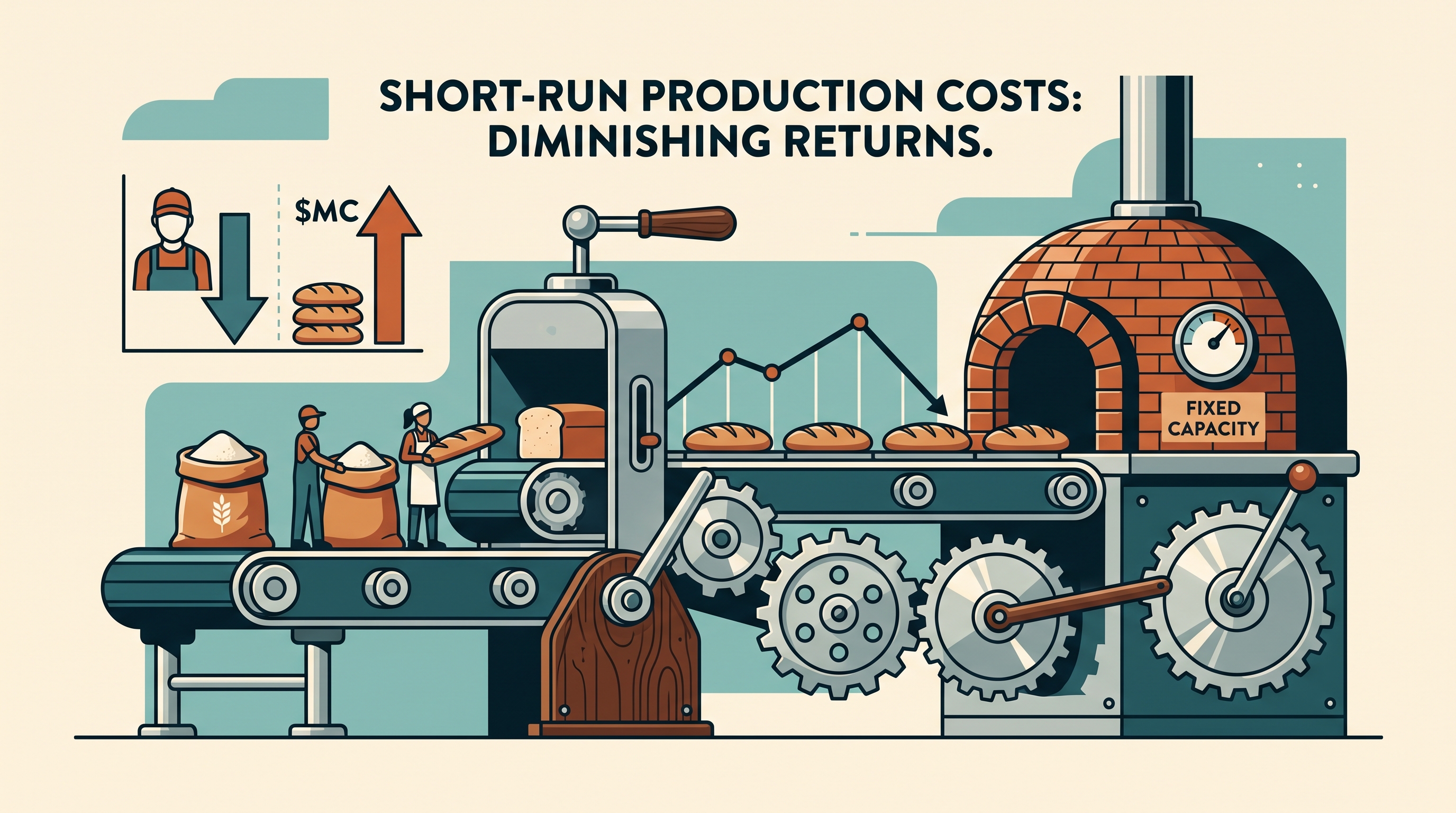
A bakery can add workers today, but it cannot instantly enlarge its ovens or building. That asymmetry creates the short run: at least one input is fixed, while other inputs are variable.
3.2 Short-Run Production Costs** [PRD]
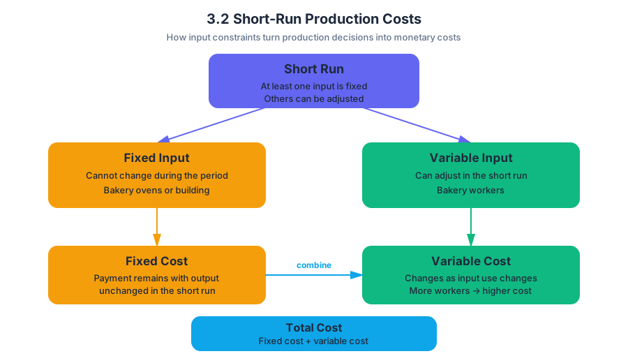
A bakery can add workers today, but it cannot instantly enlarge its ovens or building. That asymmetry creates the short run: at least one input is fixed, while other inputs are variable. A fixed input cannot be changed during the relevant short period; a variable input can be adjusted, such as the number of bakery workers.
The production function already established the relationship between inputs and output. Here, the key question is how changing a variable input changes production—and how those physical changes become monetary costs. This directly supports [PRD-1.A], especially defining terms, explaining production-cost relationships, and calculating productivity and costs; it also addresses [PRD-1.A.1], [PRD-1.A.2], and [PRD-1.A.3].
From workers to output: TP, MP, and AP
Total product, or $TP$, is the total quantity of output produced. Marginal product, or $MP$, is the additional output produced by one more unit of the variable input:
$$ MP = \frac{\Delta TP}{\Delta \text{input}} $$
Average product, or $AP$, is output per unit of the variable input:
$$ AP = \frac{TP}{\text{quantity of input}} $$
Suppose the bakery’s oven is fixed and workers are the variable input. The table shows how production changes as workers are added.
| Workers | Total product, $TP$ | Marginal product, $MP$ | Average product, $AP$ |
|---|---|---|---|
| $0$ | $0$ | — | — |
| $1$ | $10$ | $10$ | $10$ |
| $2$ | $24$ | $14$ | $12$ |
| $3$ | $42$ | $18$ | $14$ |
| $4$ | $56$ | $14$ | $14$ |
| $5$ | $65$ | $9$ | $13 |
| $6$ | $70$ | $5$ | $11.67$ |
For the fourth worker,
$$ MP_4=\frac{56-42}{4-3}=14 $$
and
$$ AP_4=\frac{56}{4}=14 $$
The third worker has the highest marginal product, so the $MP$ curve reaches its peak around that point. Because total product rises increasingly rapidly before this peak and increasingly slowly afterward, the peak of the $MP$ curve corresponds to the point of inflection on the $TP$ curve—the point where the slope of $TP$ changes from increasing to decreasing.
The $AP$ curve reaches its maximum when $MP=AP$. In the table, both equal $14$ at four workers. If $MP>AP$, the next worker pulls the average upward; if $MP<AP$, the next worker pulls the average downward.
The Law of Diminishing Marginal Returns
The Law of Diminishing Marginal Returns states that when more units of one input are employed while other inputs remain constant, the marginal product of the variable input eventually declines. The fourth, fifth, and sixth workers must share the same oven and workspace, so each additional worker contributes less extra output after the bakery becomes crowded.
Diminishing returns are eventual, not necessarily immediate. Early workers may specialize—one mixes, another shapes, and another loads trays—so $MP$ can initially rise. The common misconception is that diminishing returns means total product immediately falls. Instead, $TP$ can continue increasing while $MP$ declines; it is simply increasing at a decreasing rate.
Turning production into short-run costs
Short-run total cost has two parts:
$$ TC=TFC+TVC $$
Total fixed cost, $TFC$, does not change with output, even when $Q=0$. Rent for the bakery and the cost of its oven are examples. Total variable cost, $TVC$, changes as the firm uses more variable inputs, such as labor.
The corresponding per-unit measures are:
$$ AFC=\frac{TFC}{Q} $$
$$ AVC=\frac{TVC}{Q} $$
$$ ATC=\frac{TC}{Q} $$
Marginal cost is the additional cost of producing one more unit:
$$ MC=\frac{\Delta TC}{\Delta Q} =\frac{\Delta TVC}{\Delta Q} $$
The second equality holds because $TFC$ remains constant.
Suppose the bakery pays each worker $$20$. Moving from three to four workers raises output from $42$ to $56$ loaves, an increase of $14$ loaves, while variable cost rises by $$20$. Therefore,
$$ MC=\frac{$20}{14\text{ loaves}}\approx $1.43\text{ per loaf} $$
Why the marginal-cost curve changes shape
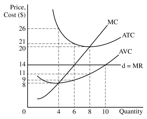
Production and cost move in opposite directions through marginal productivity. When specialization causes $MP$ to rise, each worker produces more additional output, so the cost per additional loaf can fall. Once diminishing marginal returns make $MP$ fall, the marginal-cost curve rises: more labor cost is required to produce each additional unit of output. Thus, diminishing returns yield an upward-sloping portion of $MC$, not necessarily an upward-sloping curve from the origin.
In the long run, all inputs are adjustable; the firm is no longer trapped by a fixed oven size or building. The short-run cost curves therefore describe movement along a given production capacity, while long-run analysis compares choices among different capacities.
Skill connection: Skill Category 1: Principles and Models identifies the production-cost rules; Skill Category 2: Interpretation extracts meaning from a table or graph; Skill Category 3: Manipulation calculates $MP$, $AP$, and cost measures; and Skill Category 4: Graphing and Visuals connects the shapes and positions of $TP$, $MP$, $AP$, and cost curves. On free-response questions, label axes, show substitutions, and explain the economic link rather than reporting an unexplained number.
Retrieval check: If a bakery’s $MP$ falls from $12$ to $8$ while the wage remains constant, should its $MC$ for additional output rise or fall? Answer: rise, because each worker now contributes fewer units of output, so the same wage must be spread over fewer additional units.
Source Materials
- AP Microeconomics Course and Exam Description
- AP Microeconomics Course and Exam Description Clarifications and Corrections
- AP Microeconomics Course Overview
- AP Microeconomics Course at a Glance
- AP Microeconomics Course at a Glance Poster
- AP Microeconomics
- AP Microeconomics
- AP Microeconomics Sample Syllabus 1
- (a) Calculate Hansel Hangout’s total fixed cost. Show your work.