2.6 Market Equilibrium and Consumer and Producer Surplus** `[MKT]`

2.6 Market Equilibrium and Consumer and Producer Surplus** [MKT]

A competitive market reaches equilibrium when the quantity buyers want to purchase equals the quantity sellers want to provide. At that price, the market clears: neither an unsold excess nor an unmet excess remains.

Investigative question: Why does the equilibrium price do more than balance buyers and sellers—it also determine how much benefit the market creates?

CED alignment: equilibrium and market efficiency

This topic belongs to Enduring Understanding MKT-4. Its required identifiers are:

• Learning Objective MKT-4.A: Explain how equilibrium prices and quantities are determined in competitive markets and how consumer surplus, producer surplus, and total economic surplus measure market outcomes.
• Learning Objective MKT-4.B.a: Define a surplus and shortage.
• Learning Objective MKT-4.B.b: Explain, using graphs where appropriate, how changes in underlying conditions and shocks to a competitive market can alter price, quantity, consumer surplus, and producer surplus.
• Learning Objective MKT-4.B.c: Calculate, using data from a graph or table as appropriate, changes in price, quantity, consumer surplus, and producer surplus in response to changes in market conditions or market disequilibrium.

The essential knowledge is MKT-4.A.1, MKT-4.A.2, MKT-4.A.3, MKT-4.A.4, MKT-4.A.5, MKT-4.B.1, and MKT-4.B.2. Together, these identifiers connect the supply-and-demand model to price signals, resource allocation, surplus measures, efficiency, and the movement from disequilibrium toward equilibrium.

Finding the market equilibrium

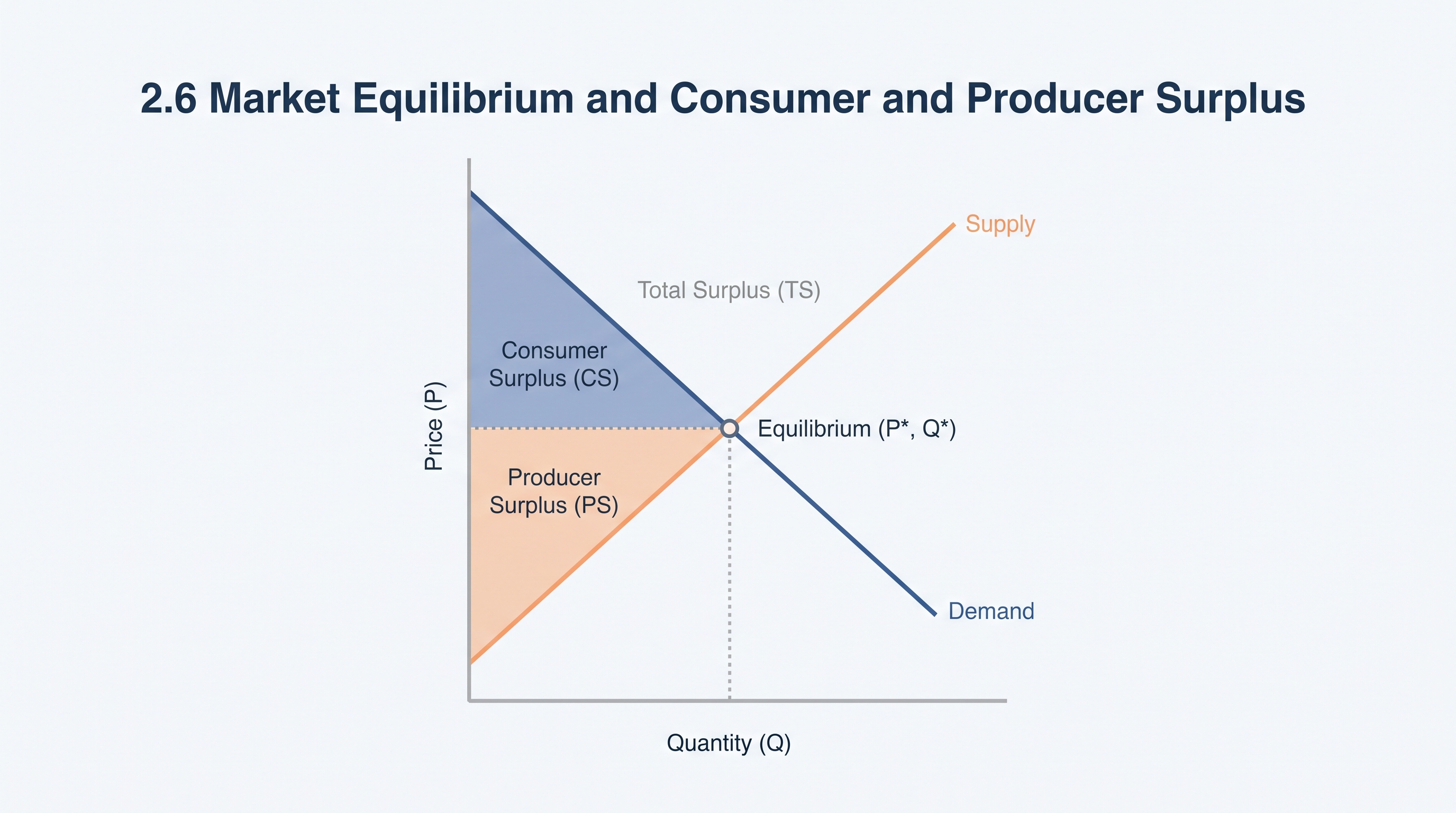
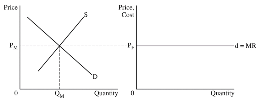
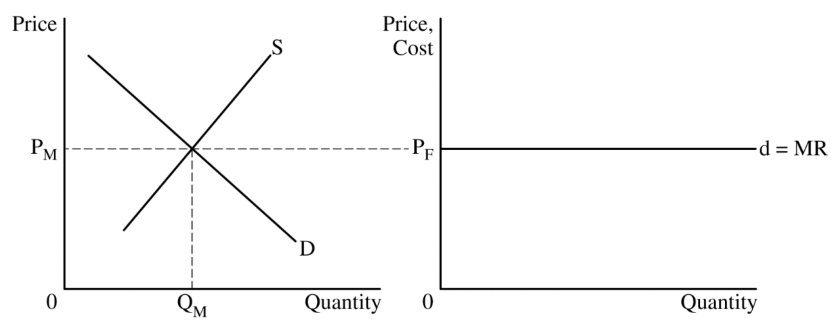
On a standard graph, price appears on the vertical axis and quantity on the horizontal axis. The downward-sloping demand curve shows the quantities buyers are willing and able to purchase at different prices; the upward-sloping supply curve shows the quantities sellers are willing and able to provide.

The intersection of demand and supply determines the equilibrium price, written as $P^$, and the equilibrium quantity, written as $Q^$. At this point,

$$Q_D = Q_S$$

For example, suppose a market has the following equilibrium data:

Price	Quantity demanded	Quantity supplied
$$4$	$80$	$40$
$$6$	$60$	$60$
$$8$	$40$	$80$

The equilibrium is therefore $P^=$6$ and $Q^=60$. At $$4$, buyers want $80$ units but sellers offer only $40$, creating a shortage of $40$ units. At $$8$, sellers offer $80$ units but buyers purchase only $40$, creating a surplus of $40$ units. The equilibrium price eliminates both gaps.

Consumer surplus: value captured by buyers

Consumer surplus is the difference between a buyer’s willingness to pay and the price actually paid. A buyer willing to pay $$10$ for a concert ticket but able to purchase it for $$6$ receives $$4$ of consumer surplus.

Consumer surplus $=$ willingness to pay $-$ actual price.

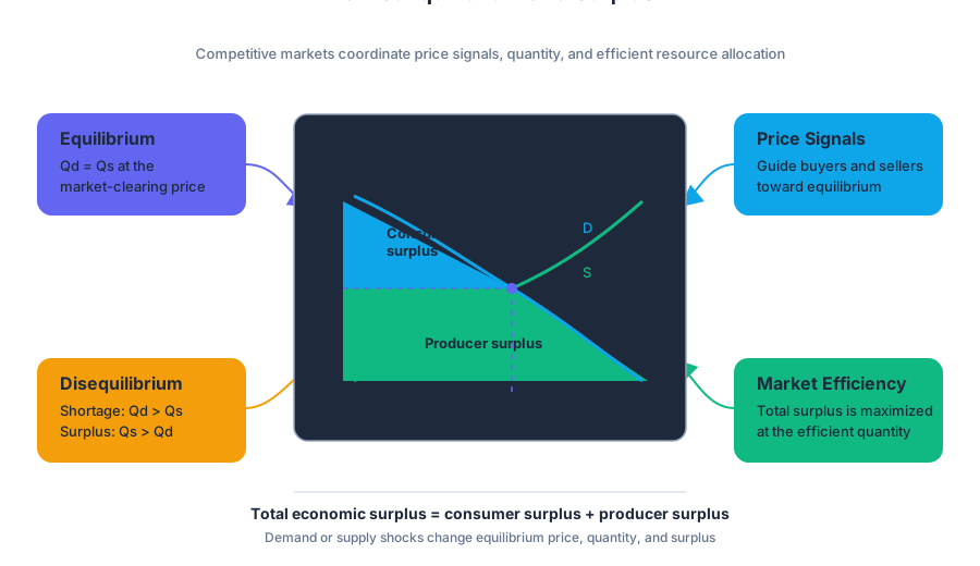
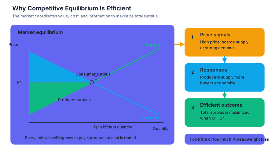
On a graph, consumer surplus is the area above the market price and below the demand curve, from zero to the equilibrium quantity. If the region is a triangle,

$$CS=\frac{1}{2}\times \text{base}\times \text{height}$$

Suppose the demand curve intercepts the price axis at $$12$, while equilibrium price is $$6$ and equilibrium quantity is $60$. Then

$$CS=\frac{1}{2}\times 60\times ($12-$6)=$180$$

The result does not mean buyers receive $$180$ in cash. It measures the total benefit buyers obtain beyond what they pay.

Producer surplus: value captured by sellers

Producer surplus is the difference between the price sellers receive and their willingness to sell, represented by the minimum price at which they would provide a unit.

Producer surplus $=$ price received $-$ willingness to sell.

On a graph, producer surplus is the area below the market price and above the supply curve, from zero to the equilibrium quantity. If the supply curve begins at a price of $$2$, equilibrium price is $$6$, and equilibrium quantity is $60$,

$$PS=\frac{1}{2}\times 60\times ($6-$2)=$120$$

The market’s total surplus is the combined benefit received by buyers and sellers:

$$TS=CS+PS$$

In this example,

$$TS=$180+$120=$300$$

Why competitive equilibrium is efficient

In the absence of market failures, perfectly competitive equilibrium maximizes total economic surplus. Every unit for which buyers’ willingness to pay is at least as large as sellers’ willingness to sell is produced and exchanged. Units that would cost more to produce than buyers value are not produced.

MKT-4.A.3 emphasizes that the equilibrium price communicates information. A high price can signal strong demand or scarce supply, encouraging producers to supply more and consumers to economize. A low price can signal weaker demand or abundant supply.

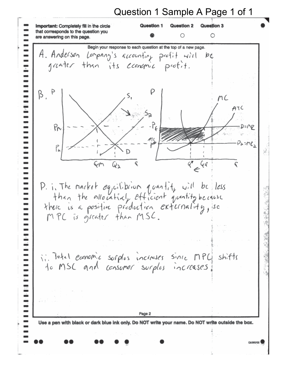
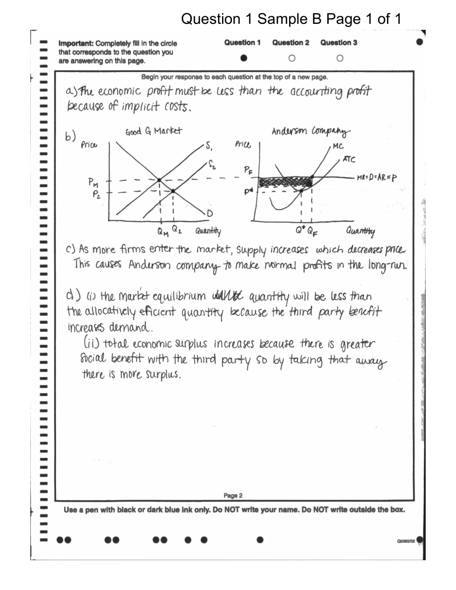
An inefficient outcome leaves mutually beneficial transactions unrealized. The resulting deadweight loss is the surplus lost because the market produces either too little or too much relative to the efficient quantity.

Skills, misconceptions, and retrieval

This topic directly exercises Skill 1.A: Define economic principles and models, when defining equilibrium, shortage, surplus, consumer surplus, producer surplus, total surplus, and deadweight loss; Skill 2.A: Determine outcomes of specific economic situations, when reading equilibrium price and quantity from a graph or table; Skill 3.A: Determine the effects of economic policies and changes in economic conditions, when calculating how a shift changes price, quantity, and surplus; and Skill 4.A: Draw graphs and visual representations, when labeling demand, supply, equilibrium, and surplus areas.

Misconception check: Consumer surplus is not total spending. Total spending is $P^\times Q^$; consumer surplus is the area above $P^*$ and below demand. Similarly, producer surplus is not total revenue: it is the area above supply and below the market price.

Retrieval check: If equilibrium price is $$8$, equilibrium quantity is $40$, demand’s price intercept is $$14$, and supply’s price intercept is $$2$, calculate $CS$, $PS$, and $TS$.

The answers are

$$CS=\frac{1}{2}\times40\times($14-$8)=$120$$

$$PS=\frac{1}{2}\times40\times($8-$2)=$120$$

$$TS=$120+$120=$240$$