3.5 Profit Maximization** `[CBA]`

3.5 Profit Maximization** [CBA]

A firm maximizes profit by expanding production only while the next unit adds more revenue than cost. The decisive question is not “How much can the firm produce?” but “Which quantity creates the largest gap between total revenue and total cost?”

Learning Objective 3.5: Explain how firms choose the quantity of output that maximizes profit.

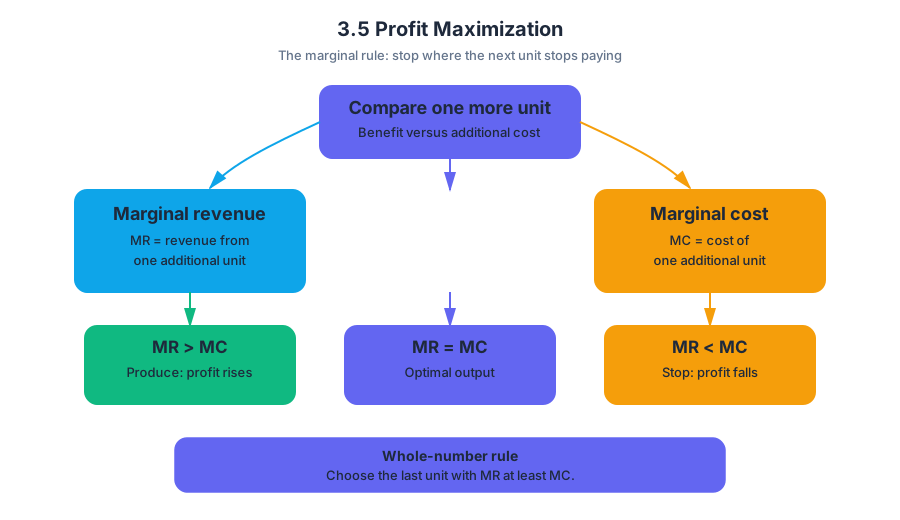
Essential Knowledge 3.5.A: A firm maximizes profit by producing the quantity of output at which marginal revenue equals marginal cost.

The marginal rule: stop where the next unit stops paying

Marginal revenue ($MR$) is the additional revenue from selling one more unit. Marginal cost ($MC$) is the additional cost of producing one more unit. If $MR > MC$, producing another unit increases profit; if $MR < MC$, that unit decreases profit.

The profit-maximizing output is therefore located where:

$$ MR = MC $$

If the exact intersection is not an available whole-number quantity, the firm produces the last unit for which $MR$ is at least as large as $MC$. This is marginal analysis: compare the benefit and cost of one additional unit, rather than comparing only totals.

Perfect competition and monopoly use the same rule—but different revenue curves

A perfectly competitive firm is a price taker, so the market price is constant for that firm. Its marginal revenue equals price:

$$ P = MR $$

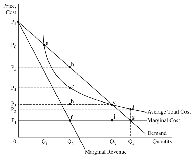
A monopolist faces a downward-sloping demand curve because it must lower price to sell more output. Its $MR$ curve also slopes downward but lies below demand: selling the additional unit requires lowering the price on units that could already have been sold.

The monopolist first finds the quantity where $MR = MC$, labels that quantity $Q_M$, and then moves vertically to the demand curve to find the price. It does not choose the price where demand intersects $MC$; that intersection identifies the socially efficient quantity, not the monopolist’s profit-maximizing quantity.

Price
  |
  |        D
  |       /
  |      /       ● P_M
  |     /        |
  |    /         |
  |---/----------|---------
  |  /           | 
  | /            |
  |/_____MR______|________ Quantity
             Q_M
             ↑
          MC intersects MR

Misconception check — “A monopolist produces where demand meets marginal cost.”
That rule confuses efficiency with private profit maximization. A monopolist chooses $Q_M$ where $MR = MC$; the price is then read from demand at $Q_M$.

Joint or collusive profit maximization

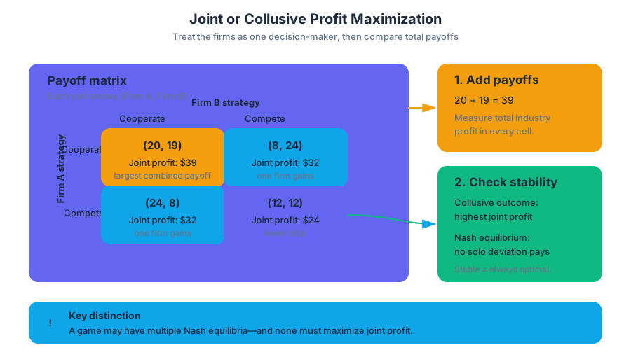
When firms coordinate as though they were one monopoly, they seek to maximize joint profit—the total payoff earned by all participating firms. In a payoff matrix, calculate joint profit by adding the two firms’ payoffs in a single cell.

For example, if one strategy combination gives Firm A a payoff of $$20$ and Firm B a payoff of $$19$:

$$ \text{Joint profit} = $20 + $19 = $39 $$

The cell with the largest combined payoff represents the collusive outcome that maximizes total industry profit. It may not be stable: one firm could gain by secretly changing strategy. A Nash equilibrium is a stable strategy combination in which no player benefits from changing strategy alone. A game can have more than one Nash equilibrium, so “stable” does not necessarily mean “unique” or “joint-profit maximizing.”

Profit maximization in the labor market: use MRP and MFC

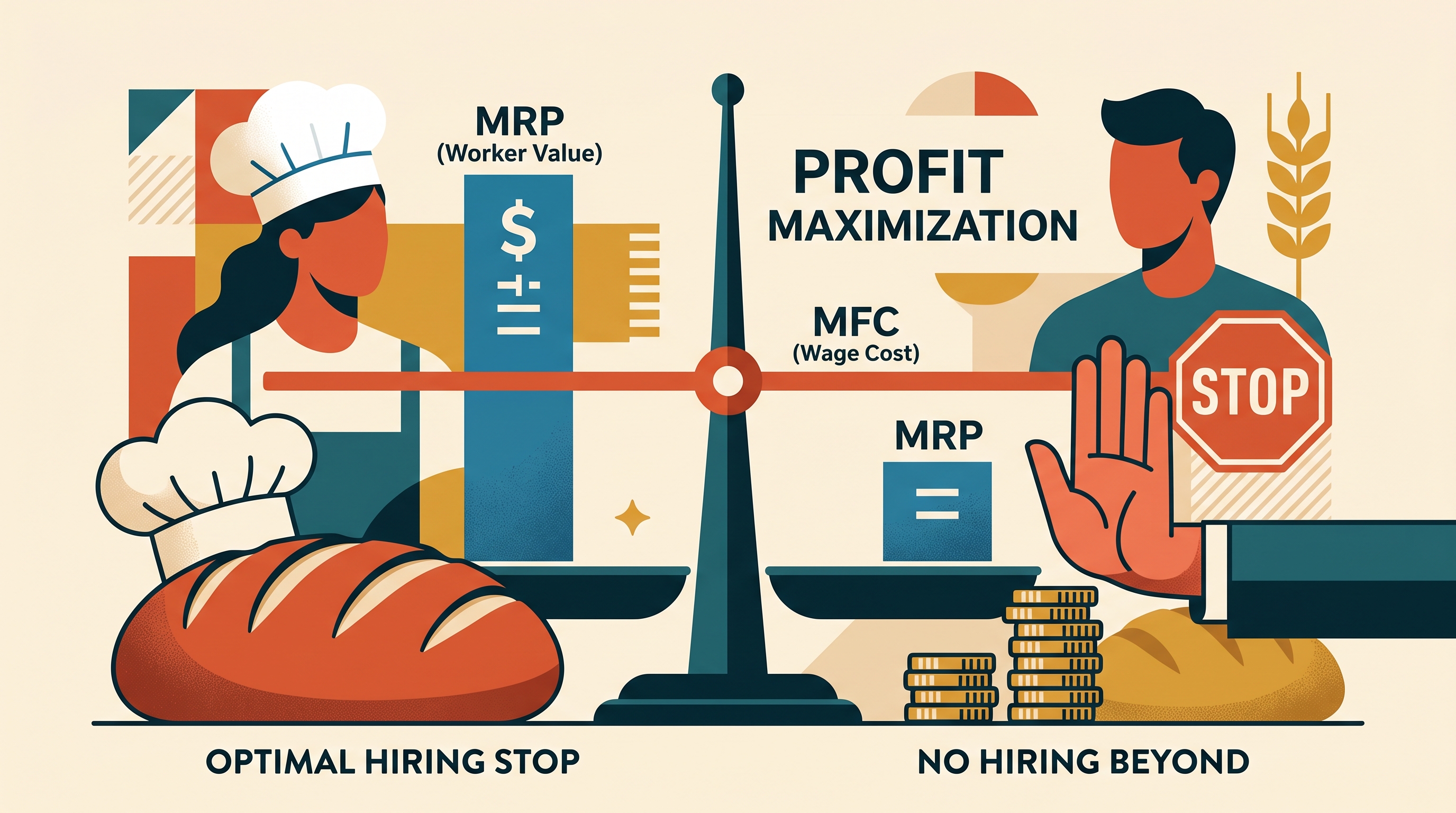
The same marginal logic determines how many workers a firm hires. Marginal revenue product ($MRP$) is the additional revenue created by one more worker:

$$ MRP = \text{Marginal Product} \times \text{Price} $$

If a worker adds $11$ jackets and each jacket sells for $$5$:

$$ MRP = 11 \times $5 = $55 $$

Marginal factor cost ($MFC$) is the additional cost of hiring one more unit of an input. In a competitive labor market, $MFC$ equals the wage. The firm hires labor up to the point where:

$$ MRP \geq MFC $$

The firm should not hire the next worker when $MRP < MFC$, because that worker adds less revenue than cost. In a production schedule with marginal products of $9$, $11$, $7$, $5$, $2$, and $1$, diminishing marginal returns begin with the third worker, because marginal product first falls from $11$ to $7$ at that point.

A fixed-cost change does not alter the profit-maximizing number of workers in the short run. Fixed cost changes total profit, but not the marginal comparison between $MRP$ and $MFC$.

Worked synthesis

Suppose a firm’s output price is $$4$, and the marginal products of successive workers are $6$, $8$, $5$, and $2$. The wage, and therefore $MFC$, is $$20$.

$$ MRP: \ $24,\ $32,\ $20,\ $8 $$

The firm hires the first three workers: each has $MRP \geq $20$. It rejects the fourth because $$8 < $20$. Diminishing marginal returns begin with the third worker because marginal product falls from $8$ to $5$.

Retrieval check

A bakery sells each loaf for $$6$. Its next three workers add $3$, $5$, and $4$ loaves, while the wage is $$24$. Which worker should be the last one hired, and when do diminishing marginal returns begin?

Answer: The $MRP$s are $$18$, $$30$, and $$24$. The bakery hires the second worker and is indifferent at the third because $MRP = MFC$; it does not hire a fourth worker if that worker’s $MRP$ is below $$24$. Diminishing marginal returns begin with the third worker because marginal product falls from $5$ to $4$.