From the free course College Algebra on Lykke
6.8 Fitting Exponential Models to Data
Key concepts: Fitting exponential or logistic models to data · Interpreting the carrying capacity · Using the model to determine the initial population · Solving an exponential equation for time · Interpreting parameters in a population-growth model
By the end of this section the student can: Build an exponential model from data; Build a logarithmic model from data; Build a logistic model from data
6.8 Fitting Exponential Models to Data
A population can grow rapidly at first and then slow dramatically as it approaches a natural limit. A rumor spreading through a school behaves this way: early on, each person can tell several others, but eventually nearly everyone has already heard it. An ordinary exponential model captures the rapid beginning, while a logistic model captures both the growth and the eventual saturation.
Fitting a model means choosing the parameters of an equation so that its graph follows observed data as closely as possible. For exponential behavior, the model often has the form
$$ y=ab^x, $$
where $a$ is the initial value and $b$ is the growth or decay factor. For growth that levels off, a logistic model is more appropriate:
$$ N(t)=\frac{L}{1+Ae^{-kt}}. $$
Here, $L$, $A$, and $k$ are parameters determined from the data or from contextual information.
Logistic model: A function of the form
$$ N(t)=\frac{L}{1+Ae^{-kt}} $$ that describes growth which begins rapidly but approaches a limiting value.
Fitting an exponential or logistic model to data
A data table gives measured input-output pairs. For example, the following values can be used to model a quantity that increases over time:
$$ \begin{array}{c|c} \text{Year} & \text{Observed value}\ \hline 1997&20.29\ 1998&25.08\ 1999&30.81\ 2000&38.75\ 2001&45.00\ 2002&49.16\ 2006&76.64\ 2007&82.47\ 2008&85.68\ 2009&89.14\ 2010&91.86\ 2011&95.28 \end{array} $$
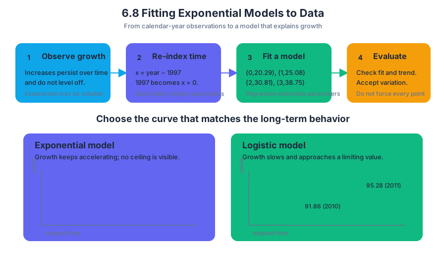
The first step is to decide which family of functions makes sense. If the data increase by approximately the same percentage over equal time intervals and do not appear to level off, an exponential model may be suitable. If the data increase at first but the increases become smaller and the values approach a ceiling, a logistic model is more appropriate.
For regression, it is usually convenient to replace a large calendar year with elapsed time. Let
$$ x=\text{year}-1997. $$
Then $1997$ becomes $x=0$, $1998$ becomes $x=1$, and so forth. The first several points become
$$ (0,20.29),\quad (1,25.08),\quad (2,30.81),\quad (3,38.75). $$
This change does not alter the data; it simply makes the model parameters easier to interpret.
A logistic regression procedure uses the data points to estimate values for $L$, $A$, and $k$. The resulting equation is then graphed together with the data. A useful fitted model should pass near the points, reproduce the observed trend, and have parameters that make sense in context. The fitted equation is not expected to pass through every measured point because real data contain variation.
For a data set such as the one above, a logistic curve rises relatively quickly and then bends toward a horizontal asymptote near its limiting value. The later observations, such as $91.86$ in $2010$ and $95.28$ in $2011$, show why a model that continues increasing without bound may eventually become unrealistic.
Worked example: organizing data for a logistic fit
Suppose the observed value in $1997$ is $20.29$ and the observed value in $2007$ is $82.47$. Convert the years to elapsed time using $x=\text{year}-1997$.
For $1997$:
$$ x=1997-1997=0. $$
For $2007$:
$$ x=2007-1997=10. $$
Therefore, the corresponding data points are
$$ (0,20.29) \quad\text{and}\quad (10,82.47). $$
The complete transformed table can then be entered into a regression tool, with $x$ as the input and the observed value as the output. The logistic regression returns an equation of the form
$$ f(x)=\frac{L}{1+Ae^{-kx}}. $$
The meaning of each parameter must be checked against the context: $L$ should represent the eventual limiting value, $A$ should determine the starting position relative to that limit, and $k$ should control how rapidly the transition occurs.
Interpreting the carrying capacity
The carrying capacity is the maximum population or level that the model predicts in the long run. In the logistic equation
$$ N(t)=\frac{L}{1+Ae^{-kt}}, $$
the carrying capacity is $L$. To see why, suppose $k>0$. As $t$ increases, $e^{-kt}$ approaches $0$. Thus,
$$ N(t)=\frac{L}{1+Ae^{-kt}} \longrightarrow \frac{L}{1+0} =L. $$
So the graph approaches the horizontal asymptote
$$ N=L. $$
For the rumor model
$$ N(t)=\frac{1200}{1+199e^{-0.625t}}, $$
the carrying capacity is
$$ L=1200. $$
This means the model predicts that approximately $1200$ people will eventually hear the rumor. It does not mean that exactly $1200$ people must hear it in reality; it means that $1200$ is the limiting value built into this model.
Important distinction: The carrying capacity is not necessarily the current population. It is the long-term level that the logistic model approaches.
Finding the initial population
The initial population is found by evaluating the model at $t=0$. In the rumor model,
$$ N(0)=\frac{1200}{1+199e^{-0.625(0)}}. $$
Because
$$ -0.625(0)=0 \quad\text{and}\quad e^0=1, $$
we obtain
$$ N(0)=\frac{1200}{1+199(1)}. $$
Simplify the denominator:
$$ 1+199(1)=1+199=200. $$
Therefore,
$$ N(0)=\frac{1200}{200}=6. $$
Thus, $6$ people started the rumor.
Worked example: interpreting the starting value
The coefficient $199$ does not represent the initial population. The initial population is found from the entire expression at $t=0$:
$$ N(0)=\frac{1200}{1+199}=6. $$
The numerator $1200$ gives the carrying capacity, while the denominator determines what fraction of that capacity is present initially. This is a common point of confusion: parameters must be interpreted from the structure of the equation, not by looking at one number in isolation.
Finding when the population reaches a specified level
A logistic model can determine the time required to reach a particular population. Half the carrying capacity in the rumor model is
$$ \frac{1200}{2}=600. $$
To find when the rumor reaches $600$ people, substitute $N(t)=600$:
$$ \frac{1200}{1+199e^{-0.625t}}=600. $$
Multiply both sides by the denominator:
$$ 1200=600\left(1+199e^{-0.625t}\right). $$
Divide both sides by $600$:
$$ \frac{1200}{600}=1+199e^{-0.625t}. $$
Therefore,
$$ 2=1+199e^{-0.625t}. $$
Subtract $1$ from both sides:
$$ 1=199e^{-0.625t}. $$
Divide by $199$:
$$ \frac{1}{199}=e^{-0.625t}. $$
Take the natural logarithm of both sides:
$$ \ln\left(\frac{1}{199}\right)=\ln\left(e^{-0.625t}\right). $$
Using $\ln(e^u)=u$ gives
$$ \ln\left(\frac{1}{199}\right)=-0.625t. $$
Since
$$ \ln\left(\frac{1}{199}\right)=-\ln(199), $$
we have
$$ -\ln(199)=-0.625t. $$
Divide by $-0.625$:
$$ t=\frac{\ln(199)}{0.625}. $$
Approximate the value:
$$ t\approx\frac{5.2933}{0.625} \approx 8.5. $$
Therefore, the rumor reaches half its carrying capacity after approximately
$$ \boxed{8.5\text{ days}}. $$
The logarithm is essential because the unknown $t$ appears in an exponent. The algebraic pattern is always the same: isolate the exponential expression, take a natural logarithm, use $\ln(e^u)=u$, and solve the resulting linear equation.
Interpreting the parameters in a population model
In the general logistic model
$$ N(t)=\frac{L}{1+Ae^{-kt}}, $$
each parameter controls a different feature:
- $L$ is the carrying capacity, or long-term limiting population.
- $A$ controls the initial position of the curve relative to $L$.
- $k$ controls the growth rate. When $k>0$, the population increases toward $L$.
- $t$ is time, and $N(t)$ is the population at that time.
The initial value can be written in terms of $L$ and $A$:
$$ N(0)=\frac{L}{1+A}. $$
For the rumor model,
$$ L=1200,\qquad A=199,\qquad k=0.625, $$
so
$$ N(0)=\frac{1200}{1+199}=6. $$
The value $k=0.625$ indicates how quickly the rumor spreads during the rapid-growth portion of the process. It is not simply the percentage increase per day; logistic growth does not maintain a constant percentage rate forever because the population is approaching its carrying capacity.
A useful special fact is that the population reaches half its carrying capacity when the denominator equals $2$:
$$ N(t)=\frac{L}{2}. $$
Starting from
$$ \frac{L}{1+Ae^{-kt}}=\frac{L}{2}, $$
divide by $L$, assuming $L\ne 0$:
$$ \frac{1}{1+Ae^{-kt}}=\frac{1}{2}. $$
Cross-multiply:
$$ 2=1+Ae^{-kt}. $$
Subtract $1$:
$$ 1=Ae^{-kt}. $$
Divide by $A$:
$$ \frac{1}{A}=e^{-kt}. $$
Take natural logarithms:
$$ \ln\left(\frac{1}{A}\right)=-kt. $$
Because $\ln(1/A)=-\ln(A)$,
$$ -\ln(A)=-kt. $$
Therefore,
$$ t=\frac{\ln(A)}{k}. $$
For $A=199$ and $k=0.625$,
$$ t=\frac{\ln(199)}{0.625}\approx 8.5. $$
This formula connects the shape parameters directly to the time at which the population reaches its midpoint.
Common modeling errors
The most common error is treating $L$ as the initial population. In a logistic equation, $L$ is the carrying capacity, while the initial population is found by calculating $N(0)$. Another error is forgetting to shift calendar years before fitting a model; using $x=1997,1998,\ldots$ can make the coefficients difficult to interpret and may create numerical problems. Finally, a logistic model should not be extrapolated automatically beyond the situation that produced the data. A fitted curve can describe the observed period well while becoming unreasonable if conditions change.
Practice problems
- For
$$ P(t)=\frac{900}{1+29e^{-0.4t}}, $$
find the carrying capacity and the initial population.
- For
$$ P(t)=\frac{900}{1+29e^{-0.4t}}, $$
find the time when the population reaches half its carrying capacity.
- A logistic data set is recorded by calendar year from $2010$ through $2020$. What substitution makes the first input value equal to $0$?
Answers:
- The carrying capacity is
$$ L=900. $$
The initial population is
$$ P(0)=\frac{900}{1+29e^0} =\frac{900}{1+29} =\frac{900}{30} =30. $$
- Half the carrying capacity is
$$ \frac{900}{2}=450. $$
Using
$$ t=\frac{\ln(A)}{k}, $$
we get
$$ t=\frac{\ln(29)}{0.4} \approx\frac{3.3673}{0.4} \approx 8.4. $$
The population reaches half its carrying capacity after approximately
$$ \boxed{8.4\text{ time units}}. $$
- Use
$$ x=\text{year}-2010. $$
Then $2010$ corresponds to $x=0$, $2011$ corresponds to $x=1$, and so on.
Content adapted from OpenStax College Algebra 2e by Jay Abramson et al., licensed CC BY 4.0.
Source Materials
Study College Algebra on Lykke
This course page is free to open: signed out, you can read its first two sections, and signing in, on any plan, opens the rest. The free Lykke Chrome extension syncs your own Canvas courses, so ChatGPT, Claude and Muse can answer from your classes and deadlines. It only reads Canvas.
Add the free extensionSign in to open every section