From the free course College Algebra on Lykke
3.3 Rates of Change and Behavior of Graphs
Key concepts: Average rate of change · Secant slope between two points · Interpreting negative rates of change · Average speed over an interval · Computing rate of change from a function formula · Increasing functions · Decreasing functions · Increasing and decreasing intervals · Local maxima · Local minima
By the end of this section the student can: Find the average rate of change of a function; Use a graph to determine where a function is increasing, decreasing, or constant; Use a graph to locate local maxima and local minima; Use a graph to locate the absolute maximum and absolute minimum
3.3 Rates of Change and Behavior of Graphs
A graph tells a story about how one quantity changes as another changes: its steepness measures how fast the output changes, while its direction reveals whether the output is rising or falling. A car’s distance graph, for example, can show not only where the car is but also whether it is traveling quickly, slowly, forward, or backward.
Average Rate of Change
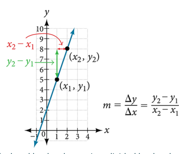
The average rate of change of a function over an interval compares the total change in the output with the total change in the input. For a function $f$ on the interval $[a,b]$, the average rate of change is
$$ \text{Average rate of change}
\frac{\text{change in output}}{\text{change in input}}
\frac{f(b)-f(a)}{b-a}. $$
The expression $f(b)-f(a)$ is the change in the function values, and $b-a$ is the length of the input interval. The order matters: the output at the right endpoint must be paired with the right endpoint in the denominator.
For $f$ on $[a,b]$,
$$ \boxed{\text{Average rate of change}=\frac{f(b)-f(a)}{b-a}} $$
provided that $a\neq b$.
On a graph, the average rate of change is the slope of the secant line joining the two points $(a,f(a))$ and $(b,f(b))$. A secant line is a line that passes through two points on a curve. It does not necessarily follow the curve between those points; instead, it summarizes the curve’s overall change across the interval.
Example: Gasoline prices
Suppose gasoline costs $$2.84$ per gallon in $2007$ and $$2.41$ per gallon in $2009$. Let $C(y)$ represent the price per gallon in year $y$. The average rate of change from $2007$ to $2009$ is
$$ \frac{C(2009)-C(2007)}{2009-2007}. $$
Substitute the given values:
$$ \frac{2.41-2.84}{2009-2007}. $$
Simplify the numerator and denominator separately:
$$ 2.41-2.84=-0.43 $$
and
$$ 2009-2007=2. $$
Therefore,
$$ \frac{-0.43}{2}=-0.215. $$
The average rate of change is
$$ \boxed{-$0.215\text{ per year}}. $$
The negative sign means that the gasoline price decreased on average over this interval. It does not mean that the price was decreasing every single day or every single year. The price could have risen during part of the interval and still have had a negative overall average change.
A negative rate of change represents a decrease, or a negative increase.
A common mistake is to report only $0.215$ and omit the negative sign. The magnitude, $$0.215$, tells how large the average change was; the sign tells its direction.
Average Speed as a Rate of Change
Average speed is another average rate of change. If $d(t)$ represents distance traveled at time $t$, then the average speed over $[t_1,t_2]$ is
$$ \text{Average speed}
\frac{d(t_2)-d(t_1)}{t_2-t_1}. $$
This formula divides the change in distance by the change in time. If distance is measured in miles and time in hours, the resulting units are miles per hour.
Example: Finding average speed
Suppose a vehicle’s distance readings show that its distance increases by $63$ miles between time $t=2$ hours and time $t=3$ hours. The average speed on $[2,3]$ is
$$ \frac{\text{change in distance}}{\text{change in time}}
\frac{63\text{ miles}}{3\text{ hours}-2\text{ hours}}. $$
Simplify the time change:
$$ 3-2=1\text{ hour}. $$
Now divide:
$$ \frac{63\text{ miles}}{1\text{ hour}}
63\text{ miles per hour}. $$
Thus, the average speed over the interval $[2,3]$ is
$$ \boxed{63\text{ miles per hour}}. $$
Average speed describes the overall distance gained per unit of time. It does not necessarily equal the vehicle’s speed at every instant. A vehicle may speed up, slow down, or stop during the interval while still averaging $63$ miles per hour.
Computing Average Rate of Change from a Function Formula
When a function is given by a formula, first evaluate the function at both endpoints, then substitute those values into the average-rate-of-change formula. Keeping the function notation visible helps prevent the common error of using endpoint values as though they were function values.
Example: A numerical interval
Find the average rate of change of
$$ f(x)=x^2+2x-8 $$
on the interval $[1,4]$.
The endpoints are $a=1$ and $b=4$. Begin by finding $f(1)$:
$$ f(1)=1^2+2(1)-8. $$
Evaluate the exponent:
$$ f(1)=1+2(1)-8. $$
Multiply:
$$ f(1)=1+2-8. $$
Simplify:
$$ f(1)=-5. $$
Now find $f(4)$:
$$ f(4)=4^2+2(4)-8. $$
Evaluate the exponent and multiplication:
$$ f(4)=16+8-8. $$
Simplify:
$$ f(4)=16. $$
Apply the formula:
$$ \frac{f(4)-f(1)}{4-1}
\frac{16-(-5)}{4-1}. $$
Simplify the numerator and denominator:
$$ \frac{16+5}{3}
\frac{21}{3}. $$
Therefore,
$$ \boxed{7} $$
is the average rate of change on $[1,4]$.
Example: A variable endpoint
$$ g(t)=t^2+3t+1 $$
on the interval $[0,a]$.
Use the endpoint formula with $0$ and $a$:
$$ \text{Average rate of change}
\frac{g(a)-g(0)}{a-0}. $$
Evaluate each function value:
$$ g(a)=a^2+3a+1 $$
and
$$ g(0)=0^2+3(0)+1. $$
Simplify $g(0)$:
$$ g(0)=0+0+1=1. $$
Substitute into the quotient:
$$ \frac{g(a)-g(0)}{a-0}
\frac{(a^2+3a+1)-1}{a-0}. $$
Simplify:
$$ \frac{a^2+3a+1-1}{a}
\frac{a^2+3a}{a}. $$
Factor the numerator:
$$ \frac{a(a+3)}{a}. $$
Cancel the common factor $a$, assuming $a\neq 0$:
$$ \boxed{a+3}. $$
The answer is an expression rather than a single number because the right endpoint has not been assigned a particular value. The algebraic cancellation is valid only when $a\neq 0$, which is also required because an interval of the form $[0,a]$ must have distinct endpoints for the average-rate formula to be defined.
Increasing and Decreasing Functions
A function’s behavior can often be read directly from its graph by moving from left to right. As the input increases, watch what happens to the output.
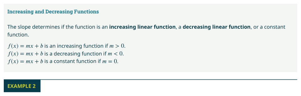
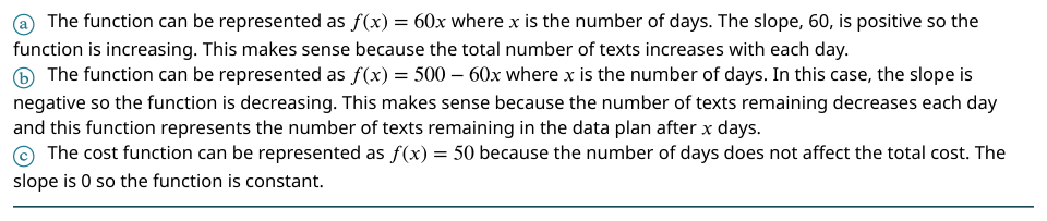
A function is increasing on an interval when larger input values produce larger function values.
In symbols, if $x_1<x_2$ and
$$ f(x_1)<f(x_2), $$
then the function is increasing between those inputs.
A function is decreasing on an interval when larger input values produce smaller function values.
$$ f(x_1)>f(x_2), $$
then the function is decreasing between those inputs.
A graph that rises as you move from left to right represents an increasing function. A graph that falls as you move from left to right represents a decreasing function. The phrase from left to right is essential: reading a graph in the opposite direction reverses the visual impression.
For example, consider
$$ f(x)=x^3-12x. $$
Its graph rises, then falls, then rises again. Therefore, it is increasing on the outer intervals and decreasing on the middle interval. The exact interval boundaries occur at the local maximum and local minimum, where the direction changes.
Local Maximum and Local Minimum
A local maximum occurs where a function changes from increasing to decreasing. The graph climbs toward the point, reaches a nearby high point, and then descends.
A local minimum occurs where a function changes from decreasing to increasing. The graph descends toward the point, reaches a nearby low point, and then climbs.
The word local means “nearby.” A local maximum is higher than nearby function values, but it might not be the highest value anywhere on the entire domain. Similarly, a local minimum is lower than nearby values, but it might not be the absolute lowest value on the entire domain.
Local extrema describe nearby behavior, not necessarily the overall highest or lowest values of a function.
For instance, a hill in the middle of a long landscape may be a local maximum even if a taller mountain exists elsewhere. A valley may be a local minimum even if the entire graph later drops lower. An absolute maximum is the greatest function value on the whole domain, while an absolute minimum is the least function value on the whole domain.
Connecting Rate of Change to Graph Behavior
The sign of an average rate of change agrees with the overall direction of a graph across the interval:
- If $\dfrac{f(b)-f(a)}{b-a}>0$, the function has increased overall.
- If $\dfrac{f(b)-f(a)}{b-a}<0$, the function has decreased overall.
- If $\dfrac{f(b)-f(a)}{b-a}=0$, the endpoint function values are equal.
A positive average rate of change does not guarantee that the function increased at every point, and a negative average rate of change does not guarantee that it decreased at every point. The average rate measures the secant line’s slope across the entire interval; local behavior may change within that interval.
Practice Problems
-
Find the average rate of change of $f(x)=3x^2-2x+1$ on $[1,3]$.
-
A cyclist travels $18$ miles between $t=2$ hours and $t=2.5$ hours. Find the cyclist’s average speed on this interval.
-
Find the average rate of change of $h(x)=x^2-4x+7$ on $[2,a]$, in simplest form.
Answers
- First evaluate:
$$ f(1)=3(1)^2-2(1)+1=3-2+1=2 $$
and
$$ f(3)=3(3)^2-2(3)+1=27-6+1=22. $$
Therefore,
$$ \frac{f(3)-f(1)}{3-1}
\frac{22-2}{2}
\frac{20}{2}
\boxed{10}. $$
- The change in time is
$$ 2.5-2=0.5\text{ hour}. $$
Thus,
$$ \text{Average speed}
\frac{18\text{ miles}}{0.5\text{ hour}}
\boxed{36\text{ miles per hour}}. $$
- Apply the formula:
$$ \frac{h(a)-h(2)}{a-2}. $$
Evaluate the function values:
$$ h(a)=a^2-4a+7 $$
and
$$ h(2)=2^2-4(2)+7=4-8+7=3. $$
Substitute:
$$ \frac{a^2-4a+7-3}{a-2}
\frac{a^2-4a+4}{a-2}. $$
Factor the numerator:
$$ \frac{(a-2)^2}{a-2}. $$
Cancel the common factor, assuming $a\neq 2$:
$$ \boxed{a-2}. $$
Content adapted from OpenStax College Algebra 2e by Jay Abramson et al., licensed CC BY 4.0.

Source Materials
Study College Algebra on Lykke
This course page is free to open: signed out, you can read its first two sections, and signing in, on any plan, opens the rest. The free Lykke Chrome extension syncs your own Canvas courses, so ChatGPT, Claude and Muse can answer from your classes and deadlines. It only reads Canvas.
Add the free extensionSign in to open every section