From the free course College Algebra on Lykke
5.3 Graphs of Polynomial Functions
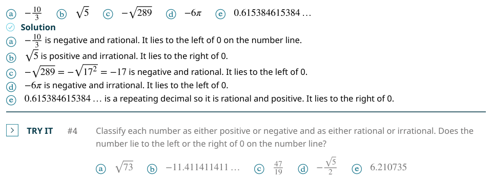
Key concepts: Identifying the degree of a polynomial · Distinguishing constants and variables in algebraic expressions · Evaluating algebraic expressions at given values · Using a graphing calculator to graph linear functions · Using the calculator’s CALC feature to find values on a graph · Rates of change and graph behavior · Function composition and the composition operator · Transformations of functions · Interpreting function inputs and outputs · Classifying numbers as rational, irrational, whole, or natural
By the end of this section the student can: Recognize characteristics of graphs of polynomial functions; Use factoring to find zeros of polynomial functions; Identify zeros and their multiplicities; Determine end behavior; Understand the relationship between degree and turning points; Graph polynomial functions; Use the Intermediate Value Theorem.
5.3 Graphs of Polynomial Functions
A polynomial graph can look complicated in the middle yet reveal its entire large-scale personality from a few facts: its zeros, the multiplicity of each zero, its leading term, and its degree. These features explain why a curve crosses or touches the $x$-axis, rises or falls at either end, and changes direction only a limited number of times.
A useful physical picture is a smooth road. A road may rise, fall, flatten, and rise again, but a polynomial graph never has a break, hole, or vertical asymptote. Its behavior is continuous, and its algebraic structure controls the shape. The main task is to translate between the factored formula and the visible features of the graph.
Recognizing Characteristics of Graphs of Polynomial Functions
A polynomial function is a function of the form
$$ f(x)=a_nx^n+a_{n-1}x^{n-1}+\cdots+a_1x+a_0, $$
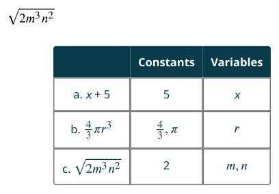
where $n$ is a nonnegative integer and the coefficients $a_n,a_{n-1},\ldots,a_0$ are real numbers, with $a_n\ne 0$. The variable is the quantity that can change, usually $x$. A constant is a fixed number, such as $7$, $-3$, or $\frac{1}{2}$.
For example, in
$$ p(x)=4x^3-7x+9, $$
$x$ is the variable, while $4$, $-7$, and $9$ are constants. The exponents $3$ and $1$ are nonnegative integers, so $p$ is a polynomial. In contrast, an expression such as $\frac{1}{x}$ is not a polynomial because it contains a negative exponent after rewriting as $x^{-1}$.
The degree of a nonzero polynomial is the greatest exponent of the variable with a nonzero coefficient. The coefficient of the highest-degree term is the leading coefficient, and that term is the leading term. A constant polynomial has degree $0$; the zero polynomial is treated separately because it has no highest nonzero power.
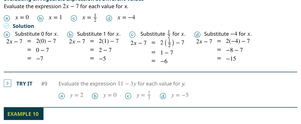
To evaluate a polynomial, substitute the given value for the variable and simplify using the order of operations. For
$$ p(x)=4x^3-7x+9, $$
evaluate $p(2)$ as follows:
$$ \begin{aligned} p(2)&=4(2)^3-7(2)+9\ &=4(8)-14+9\ &=32-14+9\ &=18+9\ &=27. \end{aligned} $$
Thus, $p(2)=27$, and the graph contains the point $(2,27)$.
Important characteristics include the $x$-intercepts, the $y$-intercept, the intervals on which the function increases or decreases, local maxima and minima, turning points, and end behavior. A common misconception is that every polynomial graph must look like a parabola. Only degree-$2$ polynomials necessarily have the basic quadratic shape; higher-degree polynomials can have several bends.
A polynomial graph can also be studied through rate of change. Between two points, the average rate of change is
$$ \frac{f(b)-f(a)}{b-a}. $$
A positive rate means the graph rises overall from $x=a$ to $x=b$; a negative rate means it falls overall. A rate of zero means the two selected function values are equal, although the graph may still rise and fall between those points.
For example, let
$$ f(x)=x^2-4x+3. $$
The average rate of change from $x=1$ to $x=3$ is
$$ \begin{aligned} f(1)&=(1)^2-4(1)+3\ &=1-4+3\ &=0, \end{aligned} $$
and
$$ \begin{aligned} f(3)&=(3)^2-4(3)+3\ &=9-12+3\ &=0. \end{aligned} $$
Therefore,
$$ \frac{f(3)-f(1)}{3-1}
\frac{0-0}{2}
$$
The graph has the same height at the two endpoints, but it decreases and then increases between them.
A graphing calculator can display a polynomial or linear function by entering the function in the graphing screen. For example, for
$$ y=2x-3, $$
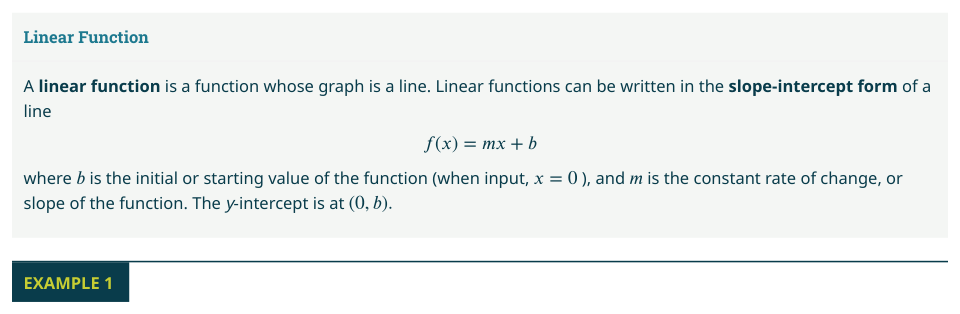
enter $2x-3$ in the expression list, use the calculator's graph key, and choose a window that displays both axes and the line. The $x$ is the variable: its value changes as the calculator traces along the graph. The numbers $2$ and $-3$ are constants: they remain fixed. The coefficient $2$ gives the line its rate of change, and the constant $-3$ gives its $y$-intercept.
The calculator's CALC feature can evaluate a function at a chosen input. For $y=2x-3$, select the CALC value option, enter $x=4$, and obtain
$$ \begin{aligned} y&=2(4)-3\ &=8-3\ &=5. \end{aligned} $$
The calculator identifies the point $(4,5)$ on the graph. This is numerical evaluation, not a replacement for understanding the algebraic rule.
Using Factoring to Find Zeros of Polynomial Functions
A zero of a polynomial function $f$ is a number $r$ for which $f(r)=0$. The corresponding point $(r,0)$ is an $x$-intercept. To find zeros, set the function equal to zero and solve. Factoring is especially useful because of the Zero Product Property:
If $AB=0$, then $A=0$ or $B=0$.
Consider
$$ f(x)=x^3-4x^2-x+4. $$
Group terms and factor each group:
$$ \begin{aligned} x^3-4x^2-x+4 &=(x^3-4x^2)+(-x+4)\ &=x^2(x-4)-1(x-4). \end{aligned} $$
Factor out the common binomial:
$$ \begin{aligned} f(x)&=(x^2-1)(x-4). \end{aligned} $$
Factor the difference of squares:
$$ \begin{aligned} x^2-1&=(x-1)(x+1), \end{aligned} $$
so
$$ f(x)=(x-1)(x+1)(x-4). $$
Set each factor equal to zero:
$$ \begin{aligned} x-1&=0 &&\Rightarrow x=1,\ x+1&=0 &&\Rightarrow x=-1,\ x-4&=0 &&\Rightarrow x=4. \end{aligned} $$
Therefore, the zeros are $x=-1$, $x=1$, and $x=4$, and the $x$-intercepts are
$$ (-1,0),\qquad (1,0),\qquad (4,0). $$
The $y$-intercept is found by setting $x=0$:
$$ \begin{aligned} f(0)&=(0-1)(0+1)(0-4)\ &=(-1)(1)(-4)\ &=4. \end{aligned} $$
Thus, the $y$-intercept is $(0,4)$.
Identifying Zeros and Their Multiplicities
If a polynomial is written in factored form,
$$ f(x)=a(x-r_1)^{m_1}(x-r_2)^{m_2}\cdots(x-r_k)^{m_k}, $$
then each $r_i$ is a zero, and the positive integer $m_i$ is its multiplicity, meaning the number of times the factor occurs. The multiplicity determines how the graph behaves at the corresponding $x$-intercept.
A zero with odd multiplicity generally produces a crossing of the $x$-axis. A zero with even multiplicity produces a touch-and-turn, or bounce, at the $x$-axis. Greater multiplicity usually makes the graph flatter near the intercept. The graph crosses or touches according to multiplicity, not merely according to whether the factor is present.
Consider
$$ g(x)=2(x+1)^3(x-2)^2. $$
The first factor gives
$$ x+1=0\quad\Rightarrow\quad x=-1, $$
with multiplicity $3$. Since $3$ is odd, the graph crosses the $x$-axis at $x=-1$.
The second factor gives
$$ x-2=0\quad\Rightarrow\quad x=2, $$
with multiplicity $2$. Since $2$ is even, the graph touches the $x$-axis and turns around at $x=2$.
The degree can also be read from the factored form:
$$ \begin{aligned} \deg(g) &=3+2\ &=5. \end{aligned} $$
The $y$-intercept is
$$ \begin{aligned} g(0) &=2(0+1)^3(0-2)^2\ &=2(1)^3(-2)^2\ &=2(1)(4)\ &=8. \end{aligned} $$
Therefore, the graph has $x$-intercepts $(-1,0)$ and $(2,0)$, $y$-intercept $(0,8)$, a crossing at $x=-1$, and a bounce at $x=2$.
Determining End Behavior
The end behavior describes what happens to $f(x)$ as $x$ increases without bound or decreases without bound. It is determined by the leading term
$$ a_nx^n. $$
For sufficiently large values of $|x|$, the leading term dominates all lower-degree terms.
The leading-term test is:
For even degree, both ends of the graph point in the same direction. A positive leading coefficient sends both ends upward; a negative leading coefficient sends both ends downward. For odd degree, the ends point in opposite directions. A positive leading coefficient sends the left end downward and the right end upward; a negative leading coefficient sends the left end upward and the right end downward.
For
$$ h(x)=-3x^5+2x^3-x+7, $$
the degree is $5$, which is odd, and the leading coefficient is $-3$, which is negative. Therefore,
$$ \begin{aligned} x\to-\infty&\quad\Rightarrow\quad h(x)\to\infty,\ x\to\infty&\quad\Rightarrow\quad h(x)\to-\infty. \end{aligned} $$
The lower-degree terms do not change this end behavior because $-3x^5$ eventually has much greater magnitude than $2x^3$, $-x$, or $7$.
For comparison, if
$$ q(x)=4x^6-x^2+10, $$
then the degree is even and the leading coefficient is positive. Thus,
$$ \begin{aligned} x\to-\infty&\quad\Rightarrow\quad q(x)\to\infty,\ x\to\infty&\quad\Rightarrow\quad q(x)\to\infty. \end{aligned} $$
Understanding the Relationship between Degree and Turning Points
A turning point is a point where a graph changes from increasing to decreasing or from decreasing to increasing. A polynomial function of degree $n$ has at most $n-1$ turning points.
The maximum number of turning points of a polynomial is one less than its degree.
The word maximum matters. A degree-$5$ polynomial can have at most $4$ turning points, but it may have fewer. Repeated zeros, unusual coefficient values, or a graph that continues in one direction can reduce the actual number.
Suppose a polynomial graph has three visible turning points. Its degree must satisfy
$$ n-1\ge 3. $$
Add $1$ to both sides:
$$ n\ge 4. $$
Therefore, the least possible degree is $4$. The graph might represent a degree-$4$, degree-$5$, or higher-degree polynomial, but it cannot represent a polynomial of degree $3$ or less.
For a concrete algebraic example, consider
$$ r(x)=x^4-4x^2. $$
Its derivative is not needed to apply the degree rule: the degree is $4$, so the graph can have at most
$$ 4-1=3 $$
turning points. Factoring reveals its intercept structure:
$$ \begin{aligned} r(x)&=x^2(x^2-4)\ &=x^2(x-2)(x+2). \end{aligned} $$
The zero $x=0$ has multiplicity $2$, so the graph touches there, while $x=-2$ and $x=2$ have multiplicity $1$, so the graph crosses there. The even degree and positive leading coefficient send both ends upward.
Graphing Polynomial Functions
To sketch a polynomial function, combine its algebraic clues in a deliberate order:
- Find the degree and leading coefficient.
- Determine the end behavior.
- Factor the polynomial when possible.
- Find each zero and its multiplicity.
- Find the $y$-intercept.
- Plot the intercepts and use multiplicity to decide whether the graph crosses or bounces.
- Draw a smooth curve with the correct end behavior.
- Check that the number of turning points does not exceed degree minus $1$.
Transformations help connect a polynomial to a familiar parent graph. In $y=f(x)+k$, the graph shifts vertically by $k$ units. In $y=f(x-h)$, it shifts horizontally right by $h$ units. A negative sign outside, $y=-f(x)$, reflects the graph across the $x$-axis; a negative sign inside, $y=f(-x)$, reflects it across the $y$-axis. A factor $a$ outside, $y=af(x)$, produces a vertical stretch when $|a|>1$ and a vertical compression when $0<|a|<1$.
For example, compare the parent function
$$ f(x)=x^3 $$
with
$$ g(x)=-2(x-1)^3+4. $$
The expression $x-1$ shifts the graph right by $1$. The factor $-2$ reflects it across the $x$-axis and stretches it vertically by a factor of $2$. The $+4$ shifts it upward by $4$. The original point $(0,0)$ becomes $(1,4)$.
Now sketch
$$ p(x)=-2(x+3)^2(x-5). $$
The degree is
$$ 2+1=3, $$
so the polynomial has odd degree. Its leading term is found from the highest-power factors:
$$ \begin{aligned} p(x)&=-2(x+3)^2(x-5)\ &\sim -2(x^2)(x)\ &=-2x^3. \end{aligned} $$
Because the degree is odd and the leading coefficient is negative,
$$ \begin{aligned} x\to-\infty&\quad\Rightarrow\quad p(x)\to\infty,\ x\to\infty&\quad\Rightarrow\quad p(x)\to-\infty. \end{aligned} $$
Find the zeros:
$$ \begin{aligned} x+3&=0 &&\Rightarrow x=-3,\ x-5&=0 &&\Rightarrow x=5. \end{aligned} $$
The zero $x=-3$ has multiplicity $2$, so the graph touches and turns at $(-3,0)$. The zero $x=5$ has multiplicity $1$, so the graph crosses at $(5,0)$.
Find the $y$-intercept:
$$ \begin{aligned} p(0) &=-2(0+3)^2(0-5)\ &=-2(3)^2(-5)\ &=-2(9)(-5)\ &=90. \end{aligned} $$
Thus, the $y$-intercept is $(0,90)$. A correct sketch begins high on the left, descends to touch the axis at $x=-3$, rises again, then crosses the axis at $x=5$ and falls toward the lower right. Since the degree is $3$, the graph has at most $2$ turning points.
Function composition combines two functions by using the output of one as the input of another:
$$ (f\circ g)(x)=f(g(x)). $$
For example, let
$$ f(x)=x^2+1 \qquad\text{and}\qquad g(x)=3x-2. $$
Then
$$ \begin{aligned} (f\circ g)(x) &=f(g(x))\ &=f(3x-2)\ &=(3x-2)^2+1\ &=(3x)^2-2(3x)(2)+2^2+1\ &=9x^2-12x+4+1\ &=9x^2-12x+5. \end{aligned} $$
At $x=2$,
$$ \begin{aligned} (f\circ g)(2) &=9(2)^2-12(2)+5\ &=9(4)-24+5\ &=36-24+5\ &=17. \end{aligned} $$
Equivalently,
$$ g(2)=3(2)-2=4, $$
and
$$ f(g(2))=f(4)=4^2+1=17. $$
Composition is useful when a polynomial transformation is described in stages, but it is not generally commutative: $f(g(x))$ and $g(f(x))$ need not be equal.
Using the Intermediate Value Theorem
The Intermediate Value Theorem states that if $f$ is continuous on the interval $[a,b]$ and $N$ lies between $f(a)$ and $f(b)$, then there is at least one number $c$ in $(a,b)$ such that
$$ f(c)=N. $$
Every polynomial is continuous everywhere, so the theorem applies to every polynomial on every closed interval.
A particularly useful consequence is the sign-change test: if
$$ f(a)<0 \qquad\text{and}\qquad f(b)>0, $$
or the signs are reversed, then $f$ has at least one zero between $a$ and $b$.
Let
$$ f(x)=x^3-x-1. $$
To show that a zero lies between $x=1$ and $x=2$, evaluate the endpoints:
$$ \begin{aligned} f(1)&=(1)^3-(1)-1\ &=1-1-1\ &=-1, \end{aligned} $$
and
$$ \begin{aligned} f(2)&=(2)^3-(2)-1\ &=8-2-1\ &=5. \end{aligned} $$
Because $f(1)<0$ and $f(2)>0$, and because $f$ is a polynomial and therefore continuous, the Intermediate Value Theorem guarantees a number $c$ with
$$ 1<c<2 $$
such that
$$ f(c)=0. $$
The theorem proves existence, but it does not by itself give the exact value of $c$.
For exam problems, distinguish carefully between “at least one zero” and “exactly one zero.” A sign change guarantees at least one zero in the interval; additional reasoning is required to prove uniqueness.
Practice Problems
- Factor and find all zeros of
$$ f(x)=x^3+2x^2-9x-18. $$
Answer:
$$ \begin{aligned} f(x) &=(x^3+2x^2)+(-9x-18)\ &=x^2(x+2)-9(x+2)\ &=(x^2-9)(x+2)\ &=(x-3)(x+3)(x+2). \end{aligned} $$
The zeros are
$$ x=3,\qquad x=-3,\qquad x=-2. $$
- Describe the zeros, multiplicities, crossing behavior, and end behavior of
$$ g(x)=-4(x-1)^2(x+2)^3. $$
Answer: The zero $x=1$ has multiplicity $2$, so the graph touches and turns there. The zero $x=-2$ has multiplicity $3$, so the graph crosses there. The degree is $5$, which is odd, and the leading coefficient is negative. Therefore,
$$ x\to-\infty\Rightarrow g(x)\to\infty, \qquad x\to\infty\Rightarrow g(x)\to-\infty. $$
- Let
$$ f(x)=x^2+3 \qquad\text{and}\qquad g(x)=2x-1. $$
Find $(f\circ g)(x)$ and evaluate $(f\circ g)(2)$.
Answer:
$$ \begin{aligned} (f\circ g)(x) &=f(g(x))\ &=f(2x-1)\ &=(2x-1)^2+3\ &=4x^2-4x+1+3\ &=4x^2-4x+4. \end{aligned} $$
Then
$$ \begin{aligned} (f\circ g)(2) &=4(2)^2-4(2)+4\ &=16-8+4\ &=12. \end{aligned} $$
Content adapted from OpenStax College Algebra 2e by Jay Abramson et al., licensed CC BY 4.0.

Source Materials
Study College Algebra on Lykke
This course page is free to open: signed out, you can read its first two sections, and signing in, on any plan, opens the rest. The free Lykke Chrome extension syncs your own Canvas courses, so ChatGPT, Claude and Muse can answer from your classes and deadlines. It only reads Canvas.
Add the free extensionSign in to open every section