From the free course College Algebra on Lykke
4.3 Fitting Linear Models to Data
Key concepts: Scatter plots and interpreting relationships between two variables · Recognizing linear and nonlinear relationships · Estimating a line of best fit by eye · Calculating slope and using the y-intercept to write a linear model · Least-squares linear regression · Using graphing utilities or calculators to find a regression line · Interpolation and extrapolation · Using a linear model to make predictions · Interpreting the domain and range of data · Evaluating whether predictions are reasonable
By the end of this section the student can: Draw and interpret scatter diagrams; Use a graphing utility to find the line of best fit; Distinguish between linear and nonlinear relations; Fit a regression line to a set of data and use the linear model to make predictions
4.3 Fitting Linear Models to Data
A scatter plot can reveal whether two measured quantities move together, whether their relationship is approximately linear, and whether a linear model is reasonable for prediction.
Scatter plots and relationships
Suppose a professor records each student’s age and final exam score. Each student contributes one ordered pair:
$$ (\text{age},\text{exam score}) $$
Plotting all of those ordered pairs gives a visual picture of whether age and exam score appear related.
A scatter plot is a graph of plotted points that may show a relationship between two sets of data.
The input variable is usually placed on the horizontal axis, or $x$-axis. The output variable is placed on the vertical axis, or $y$-axis. A scatter plot does not automatically prove that one variable causes changes in the other; it displays a pattern that may be useful for modeling.
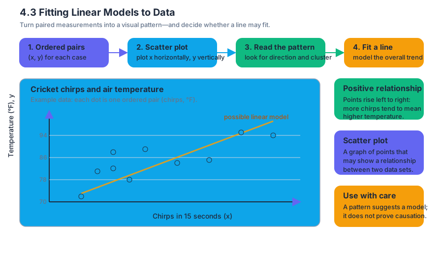
For example, cricket chirping tends to increase as air temperature increases. The data below record the number of cricket chirps in $15$ seconds and the corresponding air temperature in degrees Fahrenheit.
| Chirps in $15$ seconds, $x$ | Temperature in $\degree\text{F}$, $y$ |
|---|---|
| $20$ | $88$ |
| $16$ | $72$ |
| $26$ | $93$ |
| $23$ | $84$ |
| $19$ | $81$ |
| $20$ | $82$ |
| $22$ | $89$ |
| $28$ | $92$ |
| $24$ | $85$ |
| $18$ | $78$ |
To create the scatter plot, place chirps per $15$ seconds on the horizontal axis and temperature on the vertical axis. Then plot points such as
$$ (20,88),\quad (16,72),\quad (26,93),\quad (23,84). $$
The remaining data pairs are plotted in the same way.
The points generally rise from left to right. This indicates a positive relationship: larger numbers of chirps tend to be associated with higher temperatures. The points also appear to cluster around a straight path, suggesting that a linear model may be appropriate.
Recognizing linear and nonlinear relationships
A relationship is linear when the points in a scatter plot follow an overall straight-line pattern. The points do not have to lie exactly on one line. Real data normally contain variation, so a useful linear relationship allows points to sit above and below a central line.
A relationship is nonlinear when the points follow a noticeable curve or another pattern that a straight line cannot represent well. A curved pattern might rise rapidly and then level off, form a U-shape, or change direction.
The direction and shape of a scatter plot provide an initial assessment:
- A pattern rising from left to right suggests a positive linear relationship.
- A pattern falling from left to right suggests a negative linear relationship.
- A shapeless cloud suggests little or no relationship.
- A curved pattern suggests a nonlinear relationship.
A common misconception is that every relationship must be modeled by a line merely because the data have two variables. A line is appropriate only when the scatter plot supports an approximately straight pattern. A curved pattern requires a different type of model.
Estimating a line of best fit by eye
A line of best fit is a line that appears to fit the data in a scatter plot. Before calculating anything, we can estimate such a line by drawing it so that it passes through the middle of the data, with roughly as many points above the line as below it.
For the cricket data, a reasonable line should:
- Follow the upward direction of the points.
- Pass through the central cluster.
- Avoid being pulled toward only one unusually high or low point.
- Leave vertical deviations that are generally balanced above and below the line.
The line of best fit is not usually required to pass through every point. In fact, if the data do not lie perfectly on a line, that is impossible. The goal is to represent the overall trend rather than reproduce every observation.
Worked example: estimating a line
Suppose an eyeballed line for the cricket data passes approximately through
$$ (16,74) \quad\text{and}\quad (28,94). $$
The slope is
$$ m=\frac{94-74}{28-16}. $$
Subtract the numerators and denominators:
$$ m=\frac{20}{12}. $$
Simplify:
$$ m=\frac{5}{3}\approx 1.67. $$
Thus, the estimated temperature increases by approximately
$$ 1.67\degree\text{F} $$
for each additional cricket chirp in $15$ seconds.
Use the point $(16,74)$ to find the $y$-intercept:
$$ y=mx+b $$
$$ 74=\frac{5}{3}(16)+b. $$
Multiply:
$$ 74=\frac{80}{3}+b. $$
Subtract $\frac{80}{3}$ from both sides:
$$ b=74-\frac{80}{3}. $$
Write $74$ with denominator $3$:
$$ b=\frac{222}{3}-\frac{80}{3}. $$
Therefore,
$$ b=\frac{142}{3}\approx 47.33. $$
The estimated linear model is
$$ T(x)=\frac{5}{3}x+\frac{142}{3}, $$
where $x$ is the number of chirps in $15$ seconds and $T(x)$ is the predicted temperature in $\degree\text{F}$.
Writing a linear model from slope and intercept
A linear model has the form
$$ y=mx+b, $$
where $m$ is the slope and $b$ is the $y$-intercept. The slope describes the change in the output for each one-unit increase in the input. The intercept is the predicted output when the input equals zero.
If the slope and one point are known, substitute the point into $y=mx+b$ and solve for $b$.
The units matter. In the cricket example,
$$ m\approx 1.67\frac{\degree\text{F}}{\text{chirp per }15\text{ seconds}}. $$
This means that the predicted temperature increases by about $1.67\degree\text{F}$ for each additional chirp in $15$ seconds.
Least-squares linear regression
Eyeballing a line is useful for understanding the pattern, but different people may draw slightly different lines. Least-squares linear regression provides a precise, reproducible method.
The least-squares regression line is the line that minimizes the sum of the squared vertical differences between the observed data points and the line.
If the observed output for an input $x_i$ is $y_i$, and the line predicts $\widehat{y}_i$, then the vertical difference is
$$ y_i-\widehat{y}_i. $$
The least-squares method minimizes
$$ \sum_{i=1}^{n}\left(y_i-\widehat{y}_i\right)^2. $$
These vertical differences are called residuals. Squaring them prevents positive and negative differences from canceling and gives extra weight to points that lie far from the line.
The resulting regression line has the form
$$ \widehat{y}=mx+b, $$
where $\widehat{y}$ represents a predicted value rather than an observed value.
Finding a regression line with a calculator
Enter the input values in List $1$, often labeled $L_1$, and the output values in List $2$, often labeled $L_2$. The entries must remain paired: the first input in $L_1$ must correspond to the first output in $L_2$.
For the cricket data, enter
$$ L_1={20,16,26,23,19,20,22,28,24,18} $$
and
$$ L_2={88,72,93,84,81,82,89,92,85,78}. $$
On a graphing calculator, the general process is:
- Open the statistics-list editor.
- Enter the chirp values into $L_1$.
- Enter the temperature values into $L_2$.
- Display a scatter plot using $L_1$ for the horizontal values and $L_2$ for the vertical values.
- Select the linear regression command.
- Use $L_1$ as the input list and $L_2$ as the output list.
- Store or record the resulting equation.
A calculator produces coefficients for a model of the form
$$ \widehat{T}(x)=mx+b. $$
Always check that the lists have the same length and that the input-output pairing has not been rearranged.
Interpolation and extrapolation
Interpolation predicts a value inside the domain and range represented by the given data. Extrapolation predicts a value outside the domain or range of the given data.
Interpolation is generally more reliable because the prediction stays within the observed pattern. Extrapolation is riskier because the relationship may change beyond the data that were measured.
Worked example: cricket predictions
The cricket data contain chirp counts from $16$ through $28$ chirps in $15$ seconds. Predicting the temperature associated with $30$ chirps per $15$ seconds is an extrapolation because
$$ 30>28. $$
It is only slightly outside the observed input range, so the prediction may be reasonable if the linear trend continues nearby. However, it is still less certain than an interpolation.
Predicting the number of chirps at
$$ 40\degree\text{F} $$
is also extrapolation. The observed temperatures are approximately between $72\degree\text{F}$ and $93\degree\text{F}$, so $40\degree\text{F}$ is far outside the data range.
Moreover, crickets generally stop chirping below approximately
$$ 50\degree\text{F}. $$
A linear equation might produce a numerical answer at $40\degree\text{F}$, but that answer would not be biologically reasonable. A model should be judged not only by algebraic calculation but also by the context.
Using a fitted model for prediction
Suppose a regression calculation produces the model
$$ \widehat{P}(t)=125t+2400, $$
where $t$ is the number of years after $2010$ and $\widehat{P}(t)$ is the predicted population.
To predict the population in $2016$, first convert the calendar year to the model’s input:
$$ t=2016-2010. $$
Thus,
$$ t=6. $$
Evaluate the model:
$$ \widehat{P}(6)=125(6)+2400. $$
Multiply:
$$ \widehat{P}(6)=750+2400. $$
Add:
$$ \widehat{P}(6)=3150. $$
The model predicts a population of approximately
$$ 3150 $$
in $2016$.
The calculation is interpolation if $2016$ lies within the years used to create the model. It is extrapolation if $2016$ lies beyond those years. Even a strong regression line should not be used automatically for predictions far outside the observed data.
Practice problems
1. A scatter plot contains points that generally fall from upper left to lower right. Is the relationship positive, negative, or nonlinear?
Answer: The relationship is approximately negative because larger input values are associated with smaller output values.
2. A line of best fit passes through $(4,11)$ and $(10,23)$. Find its slope and equation.
Answer:
$$ m=\frac{23-11}{10-4} =\frac{12}{6} =2. $$
Use $y=2x+b$ and substitute $(4,11)$:
$$ 11=2(4)+b $$
$$ 11=8+b $$
$$ b=3. $$
Therefore,
$$ \boxed{y=2x+3}. $$
3. A data set uses input values from $5$ through $20$. Classify each prediction as interpolation or extrapolation:
(a) predicting the output at $12$;
(b) predicting the output at $25$.
Answer: The prediction at $12$ is interpolation because $12$ lies between $5$ and $20$. The prediction at $25$ is extrapolation because $25$ lies outside the observed input range.
Content adapted from OpenStax College Algebra 2e by Jay Abramson et al., licensed CC BY 4.0.


Source Materials
Study College Algebra on Lykke
This course page is free to open: signed out, you can read its first two sections, and signing in, on any plan, opens the rest. The free Lykke Chrome extension syncs your own Canvas courses, so ChatGPT, Claude and Muse can answer from your classes and deadlines. It only reads Canvas.
Add the free extensionSign in to open every section