From the free course College Algebra on Lykke
4.2 Modeling with Linear Functions
Key concepts: Modeling real-world situations with linear functions · Identifying changing quantities and defining descriptive variables · Using a coordinate system or sketch to represent a situation · Interpreting the vertical-axis intercept as an initial value · Interpreting the horizontal-axis intercept as the input where the output is zero · Using domain and range to describe when a model applies · Building a linear model from given information and intercepts · Evaluating a linear function to make predictions · Checking whether a mathematical result is reasonable in context · Recognizing the limitations of extrapolating beyond observed data
By the end of this section the student can: Build linear models from verbal descriptions; Model a set of data with a linear function
4.2 Modeling with Linear Functions
A linear model turns a constant-rate story into an equation that can answer practical questions: how much money remains after several weeks, how far a vehicle travels, or which company offers the lower cost. The central question is not merely “What is the equation?” but “What do the equation and its graph mean in the real situation?”
Building a Linear Model from a Verbal Description
Suppose Elan begins a vacation with $$3{,}500$ and spends $$400$ each week. The amount of money remaining changes as time passes. Because the amount decreases by the same dollar amount each week, the situation has a constant rate of change and can be modeled linearly.
A reliable modeling process is:
- Identify the changing quantities and define descriptive variables, including units.
- Read the problem carefully to identify known values, rates, and relationships.
- Determine what the problem asks you to find, solve, or interpret.
- Choose a solution pathway. This may involve a table, a graph, a formula, or careful unit analysis.
- Write a formula when necessary.
- Evaluate or solve the function.
- Decide whether the result is reasonable mathematically and in the real-world situation.
- State the result clearly, using appropriate units and a complete sentence when needed.
The model must be interpreted in context. Algebra can produce a numerical answer even when that answer describes an impossible situation, such as a negative number of weeks or a negative amount of money when borrowing is not allowed.
Step 1: Identify the variables
The two changing quantities in the vacation example are time and money. Define
$$ t=\text{number of weeks since the trip began} $$
and
$$ M(t)=\text{amount of money remaining after }t\text{ weeks}. $$
The input is $t$, measured in weeks, and the output is $M(t)$, measured in dollars. Writing the units prevents a common modeling error: confusing the input and output or attaching the rate to the wrong quantity.
Step 2: Translate the information into a formula
At $t=0$, Elan has $$3{,}500$. This is the initial value. Each week, the amount decreases by $$400$, so the rate of change is $-400$ dollars per week. Therefore,
$$ M(t)=3500-400t. $$
The same formula can be obtained from slope-intercept form,
$$ y=mx+b, $$
by identifying the slope $m=-400$ and the vertical-axis intercept $b=3500$. In this context, the function is more informative when written as $M(t)$ because the notation reminds us what the output represents.
Step 3: Evaluate the model
To find how much money remains after $5$ weeks, substitute $t=5$:
$$ M(5)=3500-400(5) $$
$$ M(5)=3500-2000 $$
$$ M(5)=1500. $$
After $5$ weeks, the model predicts that Elan has $$1{,}500$ remaining. This answer is reasonable because five weeks of spending at $$400$ per week uses $$2{,}000$, leaving $$1{,}500$ from the original $$3{,}500$.
Using a Coordinate System or Sketch
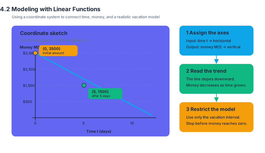
A sketch helps identify which quantity belongs on each axis. Place the input, time $t$, on the horizontal axis and the output, money $M(t)$, on the vertical axis. Important points include
$$ (0,3500), $$
which represents the initial amount, and points such as
$$ (5,1500). $$
The graph descends from left to right because the money decreases as time increases. Connecting the points with a line displays the trend, but the graph must eventually be restricted to the part that makes sense for the vacation.
Intercepts and Their Real-World Meanings
The vertical-axis intercept: initial value
The vertical-axis intercept, or $y$-intercept, is the output when the input is zero. In an appropriate real-world model, it often represents the initial value.
For the money model,
$$ M(0)=3500-400(0) $$
$$ M(0)=3500. $$
Thus, the $M$-intercept is $(0,3500)$, and its meaning is: Elan has $$3{,}500$ at the beginning of the modeled period. The intercept is not merely a point on a graph; it records the starting condition of the situation.
The horizontal-axis intercept: output equal to zero
The horizontal-axis intercept, or $x$-intercept, is the input value at which the output is zero. To find it, set the output equal to zero and solve:
$$ M(t)=0 $$
$$ 3500-400t=0 $$
$$ 3500=400t $$
$$ \frac{3500}{400}=\frac{400t}{400} $$
$$ 8.75=t. $$
The $t$-intercept is therefore $8.75$ weeks. It means that Elan will have no money left after $8.75$ weeks under this model.
This intercept also signals a limitation. The model is probably not valid after $8.75$ weeks unless Elan is allowed to use a credit card and go into debt. A formula may continue producing values after the intercept, but mathematical continuation does not guarantee real-world validity.
Domain and Range in a Real-World Model
The domain is the set of permitted input values. The range is the set of corresponding output values. In the vacation situation, negative values of $t$ do not make sense if the model begins when Elan starts spending the saved money. Also, amounts of money below zero do not make sense unless debt is explicitly allowed.
A reasonable domain is
$$ 0\leq t\leq 8.75, $$
and the corresponding range is
$$ 0\leq M(t)\leq 3500. $$
The inequalities describe the situation more accurately than the unrestricted linear function. Algebraically, $M(t)=3500-400t$ is defined for every real number $t$, but the real-world model applies only where the inputs and outputs make sense.
Building a Model from an Intercept and a Rate
Sometimes a problem gives an initial value and a constant rate rather than giving the formula directly. The method is to place the initial value in the intercept position and the rate in the slope position.
For example, suppose a tank contains $900$ liters of water initially and drains at a constant rate of $30$ liters per minute. Let $t$ be time in minutes and $V(t)$ be the volume in liters. The initial value is $900$, and the rate is $-30$ liters per minute:
$$ V(t)=900-30t. $$
To determine when the tank is empty, set the output equal to zero:
$$ V(t)=0 $$
$$ 900-30t=0 $$
$$ 900=30t $$
$$ t=30. $$
The tank empties after $30$ minutes. Since a negative time is impossible and the volume becomes negative after $30$ minutes, a reasonable domain is
$$ 0\leq t\leq 30. $$
Comparing Two Linear Cost Models
Linear models can compare competing costs. Suppose one trucking company charges a fixed fee of $$100$ plus $$2$ per mile, while Keep on Trucking, Inc. charges a fixed fee of $$200$ plus $$1$ per mile. Let $x$ represent miles driven. The cost functions are
$$ C_1(x)=100+2x $$
and
$$ C_K(x)=200+x. $$
The fixed fees are the vertical intercepts. The per-mile charges are the slopes. Company $1$ begins cheaper, but its cost grows faster because its slope is $2$ dollars per mile instead of $1$ dollar per mile.
To find when the costs are equal, set the functions equal:
$$ 100+2x=200+x $$
$$ 100+x=200 $$
$$ x=100. $$
At $100$ miles, both companies charge the same amount. Substituting into either model gives
$$ C_1(100)=100+2(100) $$
$$ C_1(100)=100+200 $$
$$ C_1(100)=300, $$
and
$$ C_K(100)=200+100=300. $$
The intersection point is $(100,300)$. It represents the real-world situation in which the two companies charge $$300$ for a $100$-mile trip. For distances greater than $100$ miles, Keep on Trucking, Inc. is cheaper because its cost grows at the slower rate. For distances less than $100$ miles, Company $1$ is cheaper because its lower initial fee outweighs its larger per-mile charge.
Interpolation, Extrapolation, and Model Breakdown
A prediction made within the domain and range of the available data is generally more reliable than a prediction outside them. Interpolation estimates a value inside the observed interval. Extrapolation estimates a value beyond that interval.
For example, if a cost model was built from data covering travel distances from $18.5$ miles through $44$ miles, estimating the cost at $30$ miles is interpolation. Estimating the cost at $100$ miles is extrapolation. The second prediction may be useful, but it is less secure because conditions may change outside the observed data.
When a model no longer applies, the situation is called model breakdown. A linear trend may work for a limited period but fail later because prices, physical limits, policies, or other conditions change. A cost model based on two years of data, for instance, should not automatically be trusted to predict costs $50$ years in the future.
Common Misconceptions
A negative output is not automatically an algebra mistake. It may be a warning that the input lies outside the model’s meaningful domain. Likewise, the $y$-intercept is not always “the value at one unit”; it is the value when the input is exactly zero. Finally, an intersection is not merely where two lines cross: in a comparison problem, it identifies the input at which the two modeled quantities are equal.
Practice Problems
-
A music account begins with $$240$ and loses $$15$ each month. Define a function for the balance and find the balance after $8$ months.
-
A taxi company charges a $$4$ starting fee and $$2.50$ per mile. Find the cost for a $12$-mile trip and explain the meaning of the vertical intercept.
-
Two delivery services have costs
$$ A(x)=50+3x $$
and
$$ B(x)=110+2x. $$
Find the distance at which their costs are equal and determine which service is cheaper for distances greater than that value.
Answers:
- The model is
$$ B(t)=240-15t. $$
Then
$$ B(8)=240-15(8)=240-120=120. $$
The balance after $8$ months is $$120$. The reasonable domain before the balance reaches zero is
$$ 0\leq t\leq 16. $$
- The model is
$$ C(x)=4+2.50x. $$
Thus,
$$ C(12)=4+2.50(12)=4+30=34. $$
The $12$-mile trip costs $$34$. The vertical intercept $$4$ is the initial starting fee.
- Set the costs equal:
$$ 50+3x=110+2x $$
$$ 50+x=110 $$
$$ x=60. $$
The costs are equal at $60$ units of distance. Since $B(x)$ has the smaller rate of change, Service $B$ is cheaper for distances greater than $60$.
A successful linear model therefore does more than produce a formula. It identifies the quantities, records the initial value and constant rate, uses intercepts and intersections to answer meaningful questions, restricts the domain and range to realistic values, and tests predictions against the limits of the situation.
Content adapted from OpenStax College Algebra 2e by Jay Abramson et al., licensed CC BY 4.0.
Source Materials
Study College Algebra on Lykke
This course page is free to open: signed out, you can read its first two sections, and signing in, on any plan, opens the rest. The free Lykke Chrome extension syncs your own Canvas courses, so ChatGPT, Claude and Muse can answer from your classes and deadlines. It only reads Canvas.
Add the free extensionSign in to open every section