From the free course AP Statistics on Lykke
3.10 Constructing a Confidence Interval for the Difference Between Two Population Proportions
Key concepts: Two-sample z-interval — estimating the gap between two proportions · Point estimate p̂₁ − p̂₂ plus or minus a margin of error · Unpooled standard error √(p̂₁q̂₁/n₁ + p̂₂q̂₂/n₂) — intervals never pool · Critical value z* determined by the confidence level · Margin of error = z* × SE, shrinking as sample sizes grow · Conditions — independent random samples or randomisation, all four counts ≥ 10
Estimating the magnitude of the difference between two population parameters allows researchers to move beyond simply asking "is there a difference?" to asking "how large is the difference?" When the data are categorical, we use a two-sample $z$-interval for $p_1 - p_2$ to estimate the…
Estimating the magnitude of the difference between two population parameters allows researchers to move beyond simply asking "is there a difference?" to asking "how large is the difference?" When the data are categorical, we use a two-sample $z$-interval for $p_1 - p_2$ to estimate the difference between two population proportions, $p_1$ and $p_2$, based on the difference between two independent sample proportions, $\hat{p}_1$ and $\hat{p}_2$. This procedure (UNC-4.D, Skill 2.C) provides a range of plausible values for the true difference in proportions at a specified confidence level.
The Anatomy of the Two-Sample $z$-Interval
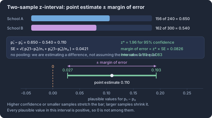
The construction of this interval follows the universal point estimate ± margin of error structure. However, because we are dealing with two independent samples, the variability of our estimate increases. The standard error of the difference reflects the combined sampling variability of both independent proportions.
The critical value, $z^*$, is determined by the desired confidence level (e.g., 1.96 for 95% confidence) and is based on the standard normal distribution. The standard error (UNC-4.F.1) is calculated using the individual sample proportions: $$SE_{\hat{p}_1 - \hat{p}_2} = \sqrt{\frac{\hat{p}_1(1-\hat{p}_1)}{n_1} + \frac{\hat{p}_2(1-\hat{p}_2)}{n_2}}$$ Note that unlike significance tests for the difference in proportions, we do not use a "pooled" proportion for confidence intervals because we are not assuming the null hypothesis ($p_1 = p_2$) is true.
Justifying the Analysis: Verification of Conditions
Before calculating the interval, we must justify that the sampling distribution of $\hat{p}_1 - \hat{p}_2$ is approximately normal and that our samples are representative (UNC-4.E, Skill 4.E). These conditions must be verified for both groups independently.
- Random: Data must come from two independent random samples or from a randomized experiment. This allows us to generalize results to the populations or make causal inferences about the treatments.
- Independent (10% Rule): When sampling without replacement from finite populations, each sample size must be less than 10% of its respective population ($n_1 < 0.10N_1$ and $n_2 < 0.10N_2$). This ensures the observations within each sample are essentially independent.
- Large Counts: The number of successes and failures in each sample must be at least 10 ($n_1\hat{p}_1 \ge 10$, $n_1(1-\hat{p}_1) \ge 10$, $n_2\hat{p}_2 \ge 10$, and $n_2(1-\hat{p}_2) \ge 10$). This condition justifies using the normal approximation for the sampling distribution (UNC-4.E.1).
Contextual Application: Public Health Study
Suppose a researcher wants to estimate the difference in the proportion of adults who exercise daily in two different cities. In City A, a random sample of 150 adults found 60 who exercise daily ($\hat{p}_A = 0.40$). In City B, a random sample of 200 adults found 100 who exercise daily ($\hat{p}_B = 0.50$).
- Identify Procedure: Two-sample $z$-interval for $p_B - p_A$.
- Verify Conditions: Both samples are random. 150 and 200 are likely less than 10% of all adults in their respective cities. Successes/Failures: City A (60, 90) and City B (100, 100) are all $\ge 10$.
- Calculate (Skill 3.E):
- Point Estimate: $0.50 - 0.40 = 0.10$
- Standard Error: $\sqrt{\frac{0.4(0.6)}{150} + \frac{0.5(0.5)}{200}} \approx 0.0534$
- Margin of Error (95%): $1.96 \times 0.0534 \approx 0.1047$
- Interval: $0.10 \pm 0.1047 \rightarrow (-0.0047, 0.2047)$
Misconception Check: The "Pooled" Trap
A common error is using a pooled proportion ($\hat{p}_c = \frac{X_1 + X_2}{n_1 + n_2}$) when constructing a confidence interval. Correction: Pooling is only appropriate for hypothesis tests where we assume $p_1 = p_2$. For confidence intervals, we are trying to estimate the difference, so we use the best available individual estimates ($\hat{p}_1$ and $\hat{p}_2$) to calculate the standard error.
Interpretation Check
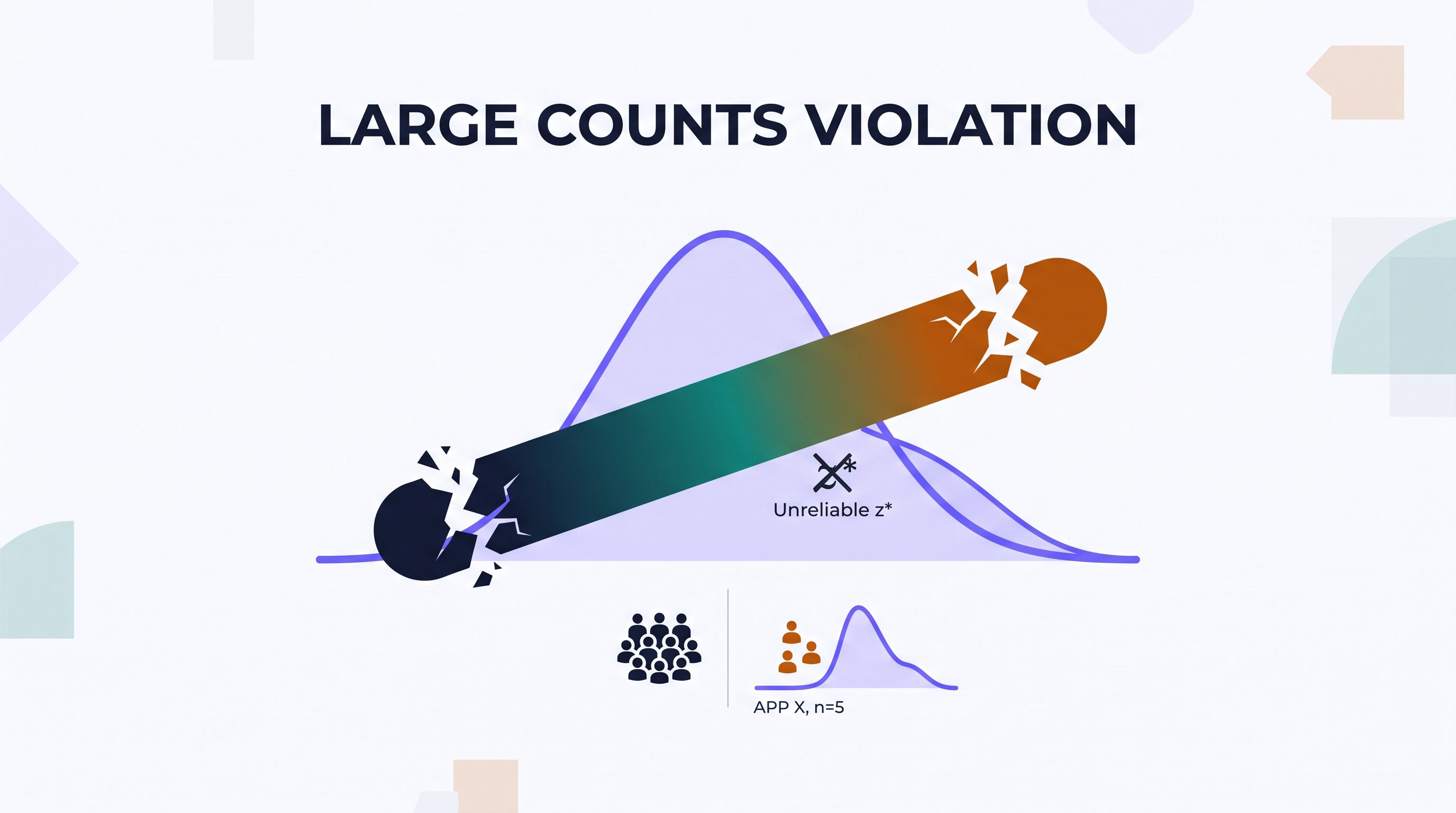
A 90% confidence interval for the difference in the proportion of teenagers who use App X versus App Y ($p_X - p_Y$) is calculated to be $(0.02, 0.12)$. If the Large Counts condition was not met for App X (e.g., only 5 teenagers used it), how would this affect the validity of the interval?
Answer Hint: If the Large Counts condition is violated, the sampling distribution of the difference in proportions may not be approximately normal. Consequently, the actual capture rate of the interval-making process might not be 90%, rendering the $z^$ critical value and the resulting interval unreliable.*