From the free course Precalculus on Lykke
Trigonometry and Sinusoidal Models
Key concepts: Unit circle identities · Inverse trigonometric functions · Law of Sines and Cosines · Sinusoidal modeling · Angle addition identities
Covers advanced trigonometric identities, the unit circle, and the application of sine and cosine laws to solve non-right triangles.
Trigonometry and Sinusoidal Models
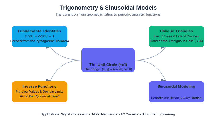
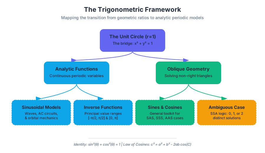
Trigonometry is often introduced as the study of right-angled triangles, but in advanced mathematics and engineering, it evolves into the study of circular functions and periodic phenomena. While a triangle is static, a circle represents rotation, and rotation over time yields a wave. This section explores the transition from geometric ratios to analytic functions, providing the toolkit necessary to model everything from the orbit of planets to the oscillation of an alternating current (AC) circuit.
The Unit Circle and Fundamental Identities
The Unit Circle is a circle with a radius of $r = 1$ centered at the origin $(0,0)$ of the Cartesian plane. It serves as the bridge between geometry and algebra. For any angle $\theta$ in standard position, the terminal side intersects the unit circle at a point $P(x, y)$.
What it is
The coordinates of $P$ are defined as:
- $x = \cos(\theta)$
- $y = \sin(\theta)$
Because the equation of the unit circle is $x^2 + y^2 = 1$, we derive the Pythagorean Identity: $$\sin^2(\theta) + \cos^2(\theta) = 1$$
Why it matters
The unit circle allows us to extend trigonometric functions beyond $90^\circ$. It defines the functions for all real numbers, creating the foundation for calculus (where $\theta$ is treated as a continuous variable in radians) and signal processing.
How it works: Special Values
The symmetry of the unit circle allows us to determine exact values for common angles ($30^\circ, 45^\circ, 60^\circ$) across all four quadrants.
| Angle (Deg) | Angle (Rad) | $\sin(\theta)$ | $\cos(\theta)$ | $\tan(\theta)$ |
|---|---|---|---|---|
| $0^\circ$ | $0$ | $0$ | $1$ | $0$ |
| $30^\circ$ | $\pi/6$ | $1/2$ | $\sqrt{3}/2$ | $\sqrt{3}/3$ |
| $45^\circ$ | $\pi/4$ | $\sqrt{2}/2$ | $\sqrt{2}/2$ | $1$ |
| $60^\circ$ | $\pi/3$ | $\sqrt{3}/2$ | $1/2$ | $\sqrt{3}$ |
| $90^\circ$ | $\pi/2$ | $1$ | $0$ | Undefined |
Inverse Trigonometric Functions and Domain Restrictions
To "undo" a trigonometric function, we use inverse functions: $\arcsin(x)$, $\arccos(x)$, and $\arctan(x)$. However, because trigonometric functions are periodic, they are not one-to-one. A single $y$-value (like $0.5$) corresponds to infinitely many $x$-values (angles).
What it is
To create a true inverse function, we must restrict the domain of the original function so that it passes the horizontal line test.
Definition: Principal Values The range of an inverse trigonometric function is restricted to a specific set of "principal values" to ensure a unique output for every input.
| Function | Notation | Domain | Range (Principal Interval) |
|---|---|---|---|
| Inverse Sine | $\sin^{-1}(x)$ | $[-1, 1]$ | $[-\pi/2, \pi/2]$ |
| Inverse Cosine | $\cos^{-1}(x)$ | $[-1, 1]$ | $[0, \pi]$ |
| Inverse Tangent | $\tan^{-1}(x)$ | $(-\infty, \infty)$ | $(-\pi/2, \pi/2)$ |
Common Pitfalls: The Quadrant Trap
A common error is assuming $\sin^{-1}(\sin(\theta)) = \theta$ for all $\theta$. This is only true if $\theta$ is within the restricted range. For example, $\sin^{-1}(\sin(150^\circ)) = 30^\circ$, because $30^\circ$ is the principal value in the allowed range that shares the same sine value as $150^\circ$.
General Triangles: Law of Sines and Law of Cosines
While basic trig handles right triangles, the Law of Sines and Law of Cosines allow us to solve for any triangle (oblique triangles).
Law of Sines
Used when we know a side and its opposite angle. $$\frac{a}{\sin A} = \frac{b}{\sin B} = \frac{c}{\sin C}$$
Law of Cosines
A generalization of the Pythagorean theorem, used when we have two sides and the included angle (SAS) or three sides (SSS). $$c^2 = a^2 + b^2 - 2ab \cos(C)$$
Mathematical Derivation: Law of Cosines
The Law of Cosines can be derived by placing a triangle on the Cartesian plane and using the distance formula.
\text{Let vertex } C \text{ be at } (0,0).
\text{Then vertex } A \text{ is at } (b, 0) \text{ and vertex } B \text{ is at } (a \cos C, a \sin C).
\text{The distance } c \text{ between } A \text{ and } B \text{ is:}
c^2 = (a \cos C - b)^2 + (a \sin C - 0)^2
c^2 = a^2 \cos^2 C - 2ab \cos C + b^2 + a^2 \sin^2 C
c^2 = a^2(\cos^2 C + \sin^2 C) + b^2 - 2ab \cos C
\text{Since } \cos^2 C + \sin^2 C = 1:
c^2 = a^2 + b^2 - 2ab \cos C
The Ambiguous Case (SSA)
When using the Law of Sines with two sides and a non-included angle (Side-Side-Angle), three possibilities exist:
- No triangle exists (the side is too short to reach).
- Exactly one triangle exists (a right triangle or only one possible orientation).
- Two distinct triangles exist (the "swinging door" effect where the side can hinge inward or outward).
| Condition ($a, b, A$) | Number of Triangles |
|---|---|
| $a < b \sin A$ | 0 |
| $a = b \sin A$ | 1 (Right Triangle) |
| $b \sin A < a < b$ | 2 (Ambiguous Case) |
| $a \ge b$ | 1 |
Sinusoidal Modeling
A sinusoid is a mathematical curve that describes a smooth periodic oscillation. It is the most efficient way to model repetitive data.
The Standard Equation
The general form of a sinusoidal function is: $$y = A \sin(B(x - C)) + D$$
Where:
- $A$ (Amplitude): The vertical stretch; half the distance between the maximum and minimum values.
- $P$ (Period): The horizontal length of one full cycle. $P = \frac{2\pi}{|B|}$.
- $C$ (Phase Shift): The horizontal displacement.
- $D$ (Vertical Shift/Midline): The average value of the function.
Modeling Workflow
To model real-world data (e.g., temperature over a year):
- Identify Midline ($D$): Calculate $\frac{\text{max} + \text{min}}{2}$.
- Identify Amplitude ($A$): Calculate $\text{max} - D$.
- Identify Period ($P$): Determine the time for one cycle (e.g., 12 months) and solve for $B = \frac{2\pi}{P}$.
- Identify Phase Shift ($C$): Find where the data starts its upward trend relative to a standard sine wave starting at the midline.
Angle Addition and Composite Identities
In many engineering applications, we need to decompose a complex wave into simpler components or rotate a vector by a specific angle. This is where Angle Addition Identities become essential.
The Core Identities
Sum and Difference Formulas
- $\sin(\alpha \pm \beta) = \sin \alpha \cos \beta \pm \cos \alpha \sin \beta$
- $\cos(\alpha \pm \beta) = \cos \alpha \cos \beta \mp \sin \alpha \sin \beta$
- $\tan(\alpha \pm \beta) = \frac{\tan \alpha \pm \tan \beta}{1 \mp \tan \alpha \tan \beta}$
Double-Angle Identities
Derived by setting $\alpha = \beta = \theta$:
- $\sin(2\theta) = 2 \sin \theta \cos \theta$
- $\cos(2\theta) = \cos^2 \theta - \sin^2 \theta = 2\cos^2 \theta - 1 = 1 - 2\sin^2 \theta$
Summary of Sinusoidal Parameters
When analyzing a waveform, the following table serves as a quick reference for relating the algebraic equation to the physical graph.
| Parameter | Algebraic Role | Graphical Effect | Physical Analogy |
|---|---|---|---|
| $A$ | Coefficient of Sine | Vertical Stretch | Volume / Brightness |
| $B$ | Frequency Factor | Horizontal Compression | Pitch / Color (Frequency) |
| $C$ | Horizontal Shift | Lateral Translation | Delay / Timing |
| $D$ | Constant Term | Vertical Translation | DC Offset / Baseline |
Advanced Applications: Fourier Analysis
While this unit focuses on single sinusoids, it is important to note that any periodic function (square waves, sawtooth waves, or human speech) can be represented as a sum of infinite sine and cosine waves. This is known as a Fourier Series. The identities learned here (specifically angle addition and product-to-sum) are the mechanics that allow us to decompose these complex signals into their constituent frequencies.
Source Materials
Study Precalculus on Lykke
This course page is free to open: signed out, you can read its first two sections, and signing in, on any plan, opens the rest. The free Lykke Chrome extension syncs your own Canvas courses, so ChatGPT, Claude and Muse can answer from your classes and deadlines. It only reads Canvas.
Add the free extensionSign in to open every section