From the free course Precalculus on Lykke
Matrices
Key concepts: Matrix multiplication · Geometric transformations · Determinants and area · Inverse matrices
Covers matrix algebra, determinants, and the use of inverse matrices to solve systems of linear equations and perform geometric transformations.
Matrices: The Engines of Linear Algebra
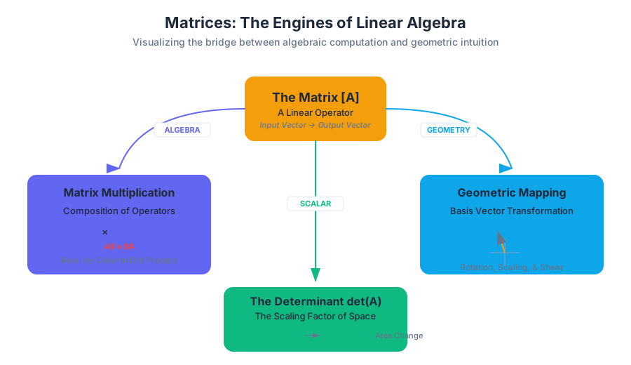
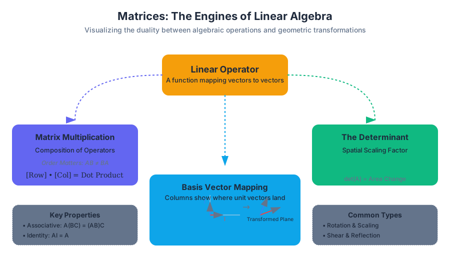
In the landscape of modern mathematics, a matrix is far more than a simple grid of numbers. While a novice might view a matrix as a static data structure—a spreadsheet of values—a mathematician or engineer views it as a linear operator. It is a machine that takes a vector and transforms it into another vector, preserving the origin and the parallelism of lines.
From the perspective of computational science, matrices are the fundamental language of the physical world. Whether you are simulating the stress on a bridge, rendering a 3D character in a video game, or training a neural network with billions of parameters, you are performing matrix operations. This article explores the mechanics of these operations, the geometric intuition behind them, and the algebraic structures that allow us to "undo" transformations.
1. Matrix Multiplication: The Composition of Operators
Matrix multiplication is the most fundamental operation in linear algebra, yet it is often the most misunderstood by beginners. Unlike addition, which is performed element-wise, multiplication is a compositional process.
1.1 The Mechanics: Row-by-Column
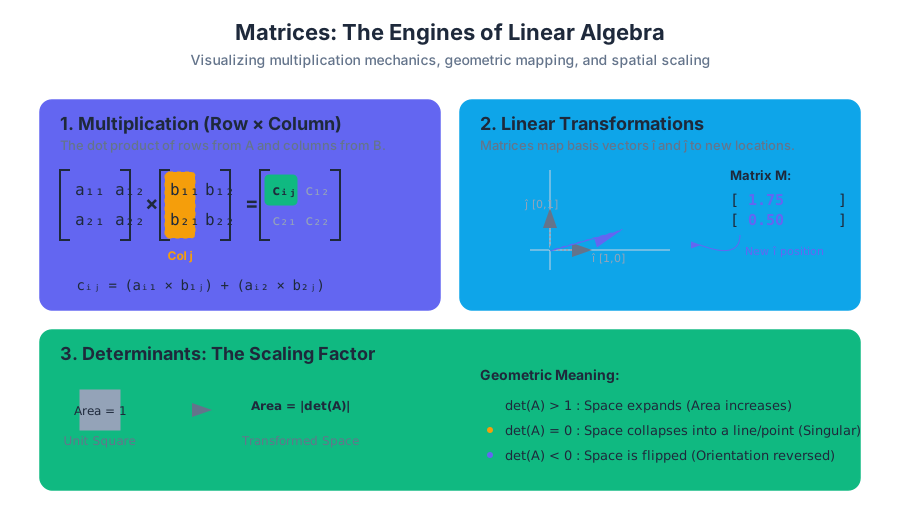
To multiply two matrices $A$ and $B$, the number of columns in $A$ must equal the number of rows in $B$. If $A$ is an $m \times n$ matrix and $B$ is $n \times p$, the resulting matrix $C$ will be $m \times p$. Each element $c_{ij}$ is the dot product of the $i$-th row of $A$ and the $j$-th column of $B$.
Definition: Matrix Multiplication For matrices $A$ (size $m \times n$) and $B$ (size $n \times p$), the product $C = AB$ is defined by: $$c_{ij} = \sum_{k=1}^{n} a_{ik}b_{kj}$$
1.2 Properties and Constraints
The most critical realization in matrix algebra is that multiplication is non-commutative. In almost all cases, $AB \neq BA$. Geometrically, this makes sense: if you rotate a cube and then slide it, you end up in a different position than if you slid it first and then rotated it.
| Property | Formula | Description |
|---|---|---|
| Non-Commutative | $AB \neq BA$ | The order of operations matters significantly. |
| Associative | $A(BC) = (AB)C$ | Grouping does not change the result. |
| Distributive | $A(B + C) = AB + AC$ | Multiplication distributes over addition. |
| Identity | $AI = IA = A$ | Multiplying by the Identity matrix leaves the matrix unchanged. |
2. Geometric Transformations: Mapping the Plane
If we treat a $2 \times 2$ matrix as a function, its input is a vector $(x, y)$ and its output is a new vector $(x', y')$. This is the foundation of computer graphics. Every matrix represents a linear transformation.
2.1 The Basis Vector Intuition
To understand what a matrix does, you only need to look at what it does to the basis vectors: $\hat{i}$ (the unit vector on the x-axis, $[1, 0]$) and $\hat{j}$ (the unit vector on the y-axis, $[0, 1]$).
If a matrix $M$ is: $$ M =
\begin{bmatrix} a & b \ c & d \end{bmatrix} $$ The first column $[a, c]^T$ tells you where $\hat{i}$ lands, and the second column $[b, d]^T$ tells you where $\hat{j}$ lands. Every other point in the plane follows them linearly.
2.2 Common 2D Transformations
By manipulating these basis vectors, we can derive standard transformation matrices.
| Transformation | Matrix Representation | Effect |
|---|---|---|
| Scaling | $\begin{bmatrix} s_x & 0 \ 0 & s_y \end{bmatrix}$ | Stretches or shrinks the plane along axes. |
| Rotation ($\theta$) | $\begin{bmatrix} \cos\theta & -\sin\theta \ \sin\theta & \cos\theta \end{bmatrix}$ | Rotates the plane counter-clockwise by $\theta$. |
| Shear (Horizontal) | $\begin{bmatrix} 1 & k \ 0 & 1 \end{bmatrix}$ | Slides the top of the plane to the right by factor $k$. |
| Reflection (X-axis) | $\begin{bmatrix} 1 & 0 \ 0 & -1 \end{bmatrix}$ | Flips the plane over the x-axis. |
2.3 Mathematical Derivation of Rotation
To derive the rotation matrix, we consider where $\hat{i} = (1, 0)$ and $\hat{j} = (0, 1)$ move when rotated by $\theta$ on the unit circle.
\text{Step 1: Rotate } \hat{i} (1, 0)
\text{New position: } (\cos\theta, \sin\theta)

\text{Step 2: Rotate } \hat{j} (0, 1)
\text{New position: } (-\sin\theta, \cos\theta)

\text{Step 3: Construct Matrix } R
R = \begin{bmatrix} \text{new } \hat{i} & \text{new } \hat{j} \end{bmatrix} = \begin{bmatrix} \cos\theta & -\sin\theta \\ \sin\theta & \cos\theta \end{bmatrix}
3. Determinants: The Scaling Factor of Space
The determinant of a matrix, denoted as $\det(A)$ or $|A|$, is a scalar value that encodes how much the transformation changes areas (in 2D) or volumes (in 3D).
3.1 Geometric Interpretation
If you take a unit square (area = 1) and apply a transformation $A$, the area of the resulting parallelogram is exactly $|\det(A)|$.
- If $\det(A) = 2$, the transformation doubles the area of any shape.
- If $\det(A) = 0.5$, the area is halved.
- If $\det(A) = 0$, the transformation collapses the space into a lower dimension (a line or a point). This means the matrix is singular and has no inverse.
- If $\det(A) < 0$, the orientation of the space has been flipped (like looking in a mirror).
3.2 Calculation Methods
For a $2 \times 2$ matrix, the calculation is straightforward: $$ \det \begin{bmatrix} a & b \ c & d \end{bmatrix}
= ad - bc $$
For a $3 \times 3$ matrix, we use Laplace Expansion (expansion by minors): $$ \det
\begin{bmatrix} a & b & c \ d & e & f \ g & h & i \end{bmatrix}
= a(ei - fh) - b(di - fg) + c(dh - eg) $$
| Determinant Value | Geometric Meaning | Algebraic Meaning |
|---|---|---|
| $\det(A) \neq 0$ | Space is preserved; no collapse. | Matrix is Invertible. |
| $\det(A) = 0$ | Space collapses (Line/Point). | Matrix is Singular (Non-invertible). |
| $\det(A) = 1$ | Area/Volume is preserved. | Transformation is Equiareal. |
| $\det(A) = -1$ | Area preserved, orientation flipped. | Reflection-like transformation. |
4. Inverse Matrices: Reversing the Transformation
If a matrix $A$ represents a transformation, the inverse matrix $A^{-1}$ represents the transformation that "undoes" $A$. If you apply $A$ and then $A^{-1}$, you return to your starting position.
4.1 The Identity Matrix
The identity matrix $I$ is the "1" of the matrix world. It has 1s on the main diagonal and 0s elsewhere. $$A A^{-1} = A^{-1} A = I$$
4.2 Finding the Inverse ($2 \times 2$ Case)
For a $2 \times 2$ matrix $A = \begin{bmatrix} a & b \ c & d \end{bmatrix}$, the inverse is: $$A^{-1} = \frac{1}{\det(A)} \begin{bmatrix} d & -b \ -c & a \end{bmatrix}$$ Observe that if $\det(A) = 0$, we would be dividing by zero, which confirms why singular matrices cannot be inverted.
5. Solving Systems of Linear Equations
One of the primary motivations for studying matrices is the ability to solve systems of equations of the form: $$a_{11}x_1 + a_{12}x_2 = b_1$$ $$a_{21}x_1 + a_{22}x_2 = b_2$$
This can be written as a single matrix equation: $AX = B$.
5.1 The Matrix Solution
If $A$ is invertible, we can solve for the vector of unknowns $X$ by multiplying both sides by $A^{-1}$: $$A^{-1}(AX) = A^{-1}B$$ $$IX = A^{-1}B$$ $$X = A^{-1}B$$
5.2 Comparison of Solving Methods
While $X = A^{-1}B$ is conceptually elegant, it is not always the most efficient way to solve a system numerically.
| Method | Best For | Complexity | Pros/Cons |
|---|---|---|---|
| Matrix Inversion | Theoretical derivation | $O(n^3)$ | Easy to write; numerically unstable for large $n$. |
| Gaussian Elimination | Small to medium systems | $O(n^3)$ | Robust; standard for manual calculation. |
| LU Decomposition | Multiple $B$ vectors | $O(n^3)$ | Efficient if $A$ stays the same but $B$ changes. |
| Iterative (Jacobi/GS) | Massive sparse matrices | $O(kn^2)$ | Used in physics simulations and "Big Data". |
6. Common Pitfalls and Advanced Concepts
6.1 The "Division" Fallacy
Students often ask, "How do I divide by a matrix?" There is no such thing as matrix division. You must use the inverse. Furthermore, because multiplication is non-commutative, you must specify if you are "pre-multiplying" or "post-multiplying."
- $AX = B \implies X = A^{-1}B$ (Correct)
- $AX = B \implies X = BA^{-1}$ (Incorrect)
6.2 Floating Point Errors
In computational practice, a determinant might not be exactly zero due to rounding errors, but it might be "effectively zero." This is known as a poorly conditioned matrix. The Condition Number of a matrix measures how sensitive the output is to small changes in the input.
6.3 Eigenvalues and Eigenvectors
Beyond basic transformations, we look for vectors that do not change direction when a transformation is applied—only their scale changes. These are eigenvectors, and their scaling factor is the eigenvalue. This is the secret sauce behind Google's PageRank algorithm and Principal Component Analysis (PCA).
Source Materials
Study Precalculus on Lykke
This course page is free to open: signed out, you can read its first two sections, and signing in, on any plan, opens the rest. The free Lykke Chrome extension syncs your own Canvas courses, so ChatGPT, Claude and Muse can answer from your classes and deadlines. It only reads Canvas.
Add the free extensionSign in to open every section