From the free course Precalculus on Lykke
Limits and Continuity
Key concepts: Estimating limits from graphs · Algebraic limit properties · The Squeeze Theorem · Intermediate Value Theorem (IVT) · Continuity
Introduces the foundational concepts of calculus, defining how functions behave as they approach specific points or infinity.
Limits and Continuity
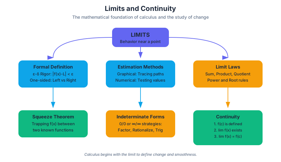
The study of calculus begins not with the derivative or the integral, but with the limit. If algebra is the study of fixed values and equations, calculus is the study of change—and the limit is the mathematical language used to describe how functions behave as they approach specific points or boundaries. Continuity, in turn, is the formalization of the intuitive idea of a "unbroken" curve. Together, these concepts provide the rigorous foundation upon which the entire edifice of modern analysis is built.
The Formal Definition of a Limit
At its core, a limit describes the value that a function $f(x)$ "approaches" as the input $x$ gets closer and closer to some value $c$. Crucially, the limit is concerned with the behavior of the function near $c$, not necessarily at $c$.
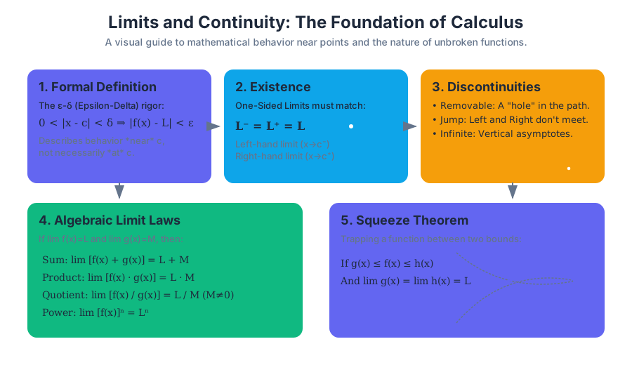
Formal Definition ($\epsilon-\delta$): We say that $\lim_{x \to c} f(x) = L$ if for every number $\epsilon > 0$, there exists a number $\delta > 0$ such that if $0 < |x - c| < \delta$, then $|f(x) - L| < \epsilon$.
This definition, pioneered by Cauchy and Weierstrass, transformed calculus from a collection of heuristic methods into a rigorous branch of mathematics. It essentially states that we can make $f(x)$ as close to $L$ as we like by making $x$ sufficiently close to $c$.
One-Sided Limits
In many cases, a function behaves differently depending on whether we approach $c$ from the left (values smaller than $c$) or the right (values larger than $c$).
- Left-hand limit: $\lim_{x \to c^-} f(x)$
- Right-hand limit: $\lim_{x \to c^2} f(x)$
A limit exists if and only if both one-sided limits exist and are equal: $$\lim_{x \to c} f(x) = L \iff \lim_{x \to c^-} f(x) = \lim_{x \to c^+} f(x) = L$$
Estimating Limits: Graphical and Numerical Approaches
Before applying algebraic rigor, we often estimate limits by observing trends.
Graphical Estimation
When looking at a graph, we trace the path of the function from both sides of $x = c$. If the "y-values" converge to a single height, that height is the limit.
- Holes (Removable Discontinuities): The limit exists even if the point is missing.
- Jumps: The left and right limits are different; the general limit does not exist (DNE).
- Vertical Asymptotes: The function grows without bound ($\infty$ or $-\infty$); the limit DNE (though we describe the direction of infinity).
Numerical Estimation
We can approximate a limit by evaluating the function at points increasingly close to $c$. For example, to find $\lim_{x \to 2} f(x)$, we might test $x = 1.9, 1.99, 1.999$ and $x = 2.1, 2.01, 2.001$.
| $x$ | $f(x) = \frac{x^2 - 4}{x - 2}$ | Observation |
|---|---|---|
| 1.9 | 3.9 | Approaching from left |
| 1.99 | 3.99 | Getting closer to 4 |
| 2.01 | 4.01 | Approaching from right |
| 2.001 | 4.001 | Getting closer to 4 |
| 2.0 | undefined | Point does not exist, but limit does |
Algebraic Limit Properties
Calculating limits by hand using the $\epsilon-\delta$ definition is cumbersome. Instead, we use Limit Laws, which allow us to break complex functions into simpler components.
The Limit Laws
Assume $\lim_{x \to c} f(x) = L$ and $\lim_{x \to c} g(x) = M$.
| Law Name | Formula |
|---|---|
| Sum/Difference | $\lim_{x \to c} [f(x) \pm g(x)] = L \pm M$ |
| Constant Multiple | $\lim_{x \to c} [k \cdot f(x)] = k \cdot L$ |
| Product | $\lim_{x \to c} [f(x) \cdot g(x)] = L \cdot M$ |
| Quotient | $\lim_{x \to c} \frac{f(x)}{g(x)} = \frac{L}{M}$, provided $M \neq 0$ |
| Power/Root | $\lim_{x \to c} [f(x)]^n = L^n$ |
Strategies for Indeterminate Forms
When direct substitution results in $0/0$ or $\infty/\infty$, the limit is in an indeterminate form. This does not mean the limit doesn't exist; it means more work is required.
- Factoring: For rational functions, factor the numerator and denominator to cancel the term causing the zero.
- Rationalization: For functions involving square roots, multiply by the conjugate.
- Trigonometric Identities: Use identities like $\lim_{\theta \to 0} \frac{\sin \theta}{\theta} = 1$ to simplify expressions.
The Squeeze Theorem
The Squeeze Theorem (also known as the Sandwich Theorem) is used to find the limit of a function that is difficult to evaluate directly by "trapping" it between two functions whose limits are known.
Theorem: If $g(x) \leq f(x) \leq h(x)$ for all $x$ in an open interval containing $c$ (except possibly at $c$), and if: $$\lim_{x \to c} g(x) = \lim_{x \to c} h(x) = L$$ then: $$\lim_{x \to c} f(x) = L$$
Classic Example: $x^2 \sin(1/x)$
Consider $\lim_{x \to 0} x^2 \sin(\frac{1}{x})$.
- We know that $-1 \leq \sin(\frac{1}{x}) \leq 1$ for all $x \neq 0$.
- Multiplying by $x^2$ (which is always $\geq 0$), we get: $-x^2 \leq x^2 \sin(\frac{1}{x}) \leq x^2$.
- Since $\lim_{x \to 0} (-x^2) = 0$ and $\lim_{x \to 0} (x^2) = 0$, by the Squeeze Theorem, $\lim_{x \to 0} x^2 \sin(\frac{1}{x}) = 0$.
Continuity
Continuity is the mathematical formalization of "smoothness." A function is continuous if you can draw its graph without lifting your pencil. However, for calculus, we need a point-specific definition.
The Three-Part Test for Continuity
A function $f(x)$ is continuous at a point $c$ if and only if:
- $f(c)$ is defined (the point exists).
- $\lim_{x \to c} f(x)$ exists (the left and right limits match).
- $\lim_{x \to c} f(x) = f(c)$ (the limit matches the actual value).
If any of these conditions fail, the function is discontinuous at $c$.
Types of Discontinuities
| Type | Description | Graphical Feature | Removable? |
|---|---|---|---|
| Removable | Limit exists, but $f(c)$ is either undefined or different. | A "hole" in the graph. | Yes (by redefining $f(c)$). |
| Jump | Left and right limits exist but are not equal. | A vertical break between segments. | No. |
| Infinite | Function approaches $\pm \infty$ as $x \to c$. | A vertical asymptote. | No. |
| Oscillating | Function oscillates infinitely fast as it nears $c$. | Dense "zig-zags" (e.g., $\sin(1/x)$). | No. |
/* Mathematical derivation of continuity for a piecewise function */
/* Objective: Find 'k' such that f(x) is continuous at x = 2 */

f(x) = {
  x^2 + k,  if x <= 2
  3x - 1,   if x > 2
}

Step 1: Find the left-hand limit as x -> 2
lim_{x -> 2-} f(x) = 2^2 + k = 4 + k

Step 2: Find the right-hand limit as x -> 2
lim_{x -> 2+} f(x) = 3(2) - 1 = 5

Step 3: Set limits equal for continuity
4 + k = 5
k = 1
The Intermediate Value Theorem (IVT)
The Intermediate Value Theorem is an "existence theorem." It doesn't tell you where a value is, but it guarantees that a value must exist under certain conditions.
Theorem: If $f$ is continuous on the closed interval $[a, b]$, and $N$ is any number between $f(a)$ and $f(b)$ (where $f(a) \neq f(b)$), then there exists at least one number $c$ in $(a, b)$ such that $f(c) = N$.
Why It Matters: Root Finding
The most common application of IVT is proving that a function has a root (a zero) in a given interval. If $f(a)$ is negative and $f(b)$ is positive, and $f$ is continuous, there must be some $c$ between $a$ and $b$ where $f(c) = 0$. This is the logic behind the Bisection Method used in computer science to solve equations.
Pitfall: Continuity is Mandatory
If a function is not continuous, the IVT does not apply. A step function can "jump" over the value $N$ without ever actually equaling it.
Infinite Limits and Asymptotes
Limits also describe the "end behavior" of functions or their behavior near singularities.
Vertical Asymptotes
If $f(x)$ approaches $\infty$ or $-\infty$ as $x$ approaches $c$ from either side, the line $x = c$ is a vertical asymptote. This typically occurs in rational functions when the denominator is zero and the numerator is non-zero.
Limits at Infinity (Horizontal Asymptotes)
We use $\lim_{x \to \infty} f(x)$ to describe what happens to a function as $x$ grows very large.
- If the limit is a finite number $L$, then $y = L$ is a horizontal asymptote.
- For rational functions $f(x) = \frac{P(x)}{Q(x)}$:
- If degree($P$) < degree($Q$), the limit is 0.
- If degree($P$) = degree($Q$), the limit is the ratio of leading coefficients.
- If degree($P$) > degree($Q$), the limit is $\pm \infty$ (slant or no horizontal asymptote).
Common Pitfalls and Misconceptions
- Confusing $f(c)$ with the Limit: Students often think that if $f(c)$ is undefined, the limit doesn't exist. Remember: the limit is about the neighborhood, not the point.
- Assuming $0/0$ is Zero or One: $0/0$ is an indeterminate form. It could be $5, -2, \infty$, or not exist at all. You must use algebraic manipulation.
- Ignoring One-Sided Limits: For piecewise functions or functions with absolute values, you must check both sides. If they don't match, the general limit DNE.
- Misapplying IVT: Forgetting to check if the function is continuous on the entire closed interval. A single point of discontinuity between $a$ and $b$ invalidates the theorem.
Source Materials
Study Precalculus on Lykke
This course page is free to open: signed out, you can read its first two sections, and signing in, on any plan, opens the rest. The free Lykke Chrome extension syncs your own Canvas courses, so ChatGPT, Claude and Muse can answer from your classes and deadlines. It only reads Canvas.
Add the free extensionSign in to open every section