Graphical Analysis of Motion

Graphical Analysis of Motion

In the study of kinematics, graphical analysis serves as a bridge between abstract mathematical models and physical reality. While algebraic equations provide precise solutions for idealized scenarios, graphs offer a continuous, visual narrative of an object's behavior over time. For engineers and physicists, the ability to "read" a graph is equivalent to performing calculus by sight: the slope represents a derivative, and the area under a curve represents an integral.

The Fundamental Kinematic Hierarchy

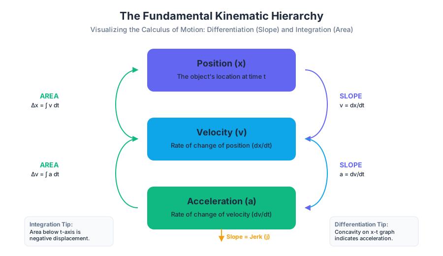
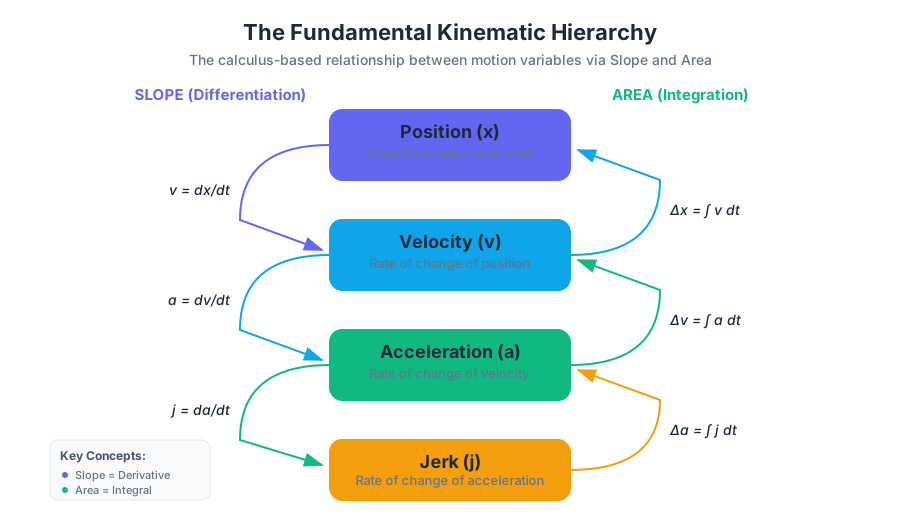
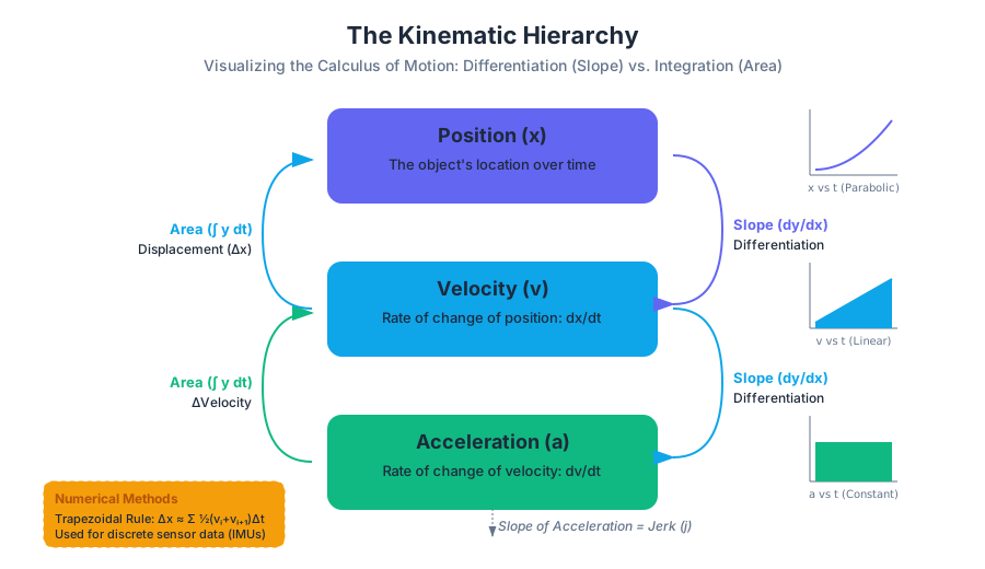
To master graphical analysis, one must understand the hierarchical relationship between position ($x$), velocity ($v$), and acceleration ($a$). These variables are linked through time ($t$) via the operations of differentiation and integration.

Graph Type	Slope ($dy/dx$)	Area Under Curve ($\int y , dt$)
Position vs. Time ($x$ vs. $t$)	Velocity ($v$)	No standard physical significance
Velocity vs. Time ($v$ vs. $t$)	Acceleration ($a$)	Displacement ($\Delta x$)
Acceleration vs. Time ($a$ vs. $t$)	Jerk ($j$)	Change in Velocity ($\Delta v$)

---

Position-Time Graphs ($x$ vs. $t$)

The Position-Time Graph is the most intuitive representation of motion. It maps an object's coordinate on a specific axis against the progression of time.

1. Interpreting the Slope

The slope of a position-time graph at any point $t$ is the instantaneous velocity $v(t)$.

Theorem: For a function $x(t)$, the velocity is defined as $v = \lim_{\Delta t \to 0} \frac{\Delta x}{\Delta t} = \frac{dx}{dt}$.

• Linear Slope: Indicates constant velocity. If the line is straight, the object is not accelerating.
• Curvature (Concavity): Indicates acceleration.
  • Concave Up (Parabolic): Positive acceleration (velocity is becoming more positive).
  • Concave Down: Negative acceleration (velocity is becoming more negative).
• Zero Slope: A horizontal line indicates the object is at rest ($v = 0$).

2. Distance vs. Displacement

A common pitfall in graphical analysis is conflating distance (a scalar) with displacement (a vector).

• Displacement ($\Delta x$): The change in position, calculated as $x_{final} - x_{initial}$. On a graph, this is simply the difference in the y-values between two points.
• Total Distance: The sum of the absolute values of all path segments. If an object moves from $x=0$ to $x=10$ and back to $x=5$, the displacement is $5$, but the distance is $15$.

---

Velocity-Time Graphs ($v$ vs. $t$)

The Velocity-Time Graph is arguably the most powerful tool in kinematics because it encodes information about position, velocity, and acceleration simultaneously.

1. Slope as Acceleration

The gradient of the $v$ vs. $t$ curve represents the instantaneous acceleration.

• A positive slope means the object is accelerating in the positive direction.
• A negative slope means the object is accelerating in the negative direction (often called deceleration, though this term can be ambiguous if the object is already moving in the negative direction).

2. Area as Displacement

The definite integral of the velocity function with respect to time yields the displacement. $$\Delta x = \int_{t_1}^{t_2} v(t) , dt$$ In a piecewise linear graph (composed of triangles and rectangles), we calculate this area using basic geometry.

Shape on Graph	Motion Description	Area Calculation
Rectangle	Constant Velocity	$v \times \Delta t$
Triangle	Constant Acceleration (starting from rest or ending at rest)	$\frac{1}{2} (v_{max} \times \Delta t)$
Trapezoid	Constant Acceleration (between two non-zero velocities)	$\frac{1}{2} (v_1 + v_2) \times \Delta t$

3. The "Negative Area" Problem

When the velocity curve dips below the t-axis (negative y-values), the object is moving in the negative direction.

• Net Displacement: Subtract the area below the axis from the area above the axis.
• Total Distance: Add the absolute values of all areas.

---

Computational Implementation: Discrete Integration

In real-world engineering, such as processing data from an IMU (Inertial Measurement Unit), we do not have continuous functions. Instead, we have discrete data points. We use numerical methods like the Trapezoidal Rule to derive displacement from velocity samples.

import numpy as np

def calculate_kinematics(time_series, velocity_series):
    """
    Computes displacement and acceleration from discrete velocity data.
    
    Args:
        time_series (np.array): Time stamps in seconds.
        velocity_series (np.array): Velocity samples in m/s.
        
    Returns:
        displacement (float): Total net displacement.
        acceleration (np.array): Instantaneous acceleration between samples.
    """
    # Calculate acceleration using central differences (slope)
    # a = dv/dt
    acceleration = np.diff(velocity_series) / np.diff(time_series)
    
    # Calculate displacement using the Trapezoidal Rule (area under curve)
    # dx = integral(v dt)
    displacement = np.trapz(velocity_series, time_series)
    
    # Calculate total distance (integral of absolute velocity)
    total_distance = np.trapz(np.abs(velocity_series), time_series)
    
    return displacement, total_distance, acceleration

# Example Data: A car accelerating then braking
t = np.array([0, 2, 4, 6, 8])
v = np.array([0, 10, 20, 10, 0])

disp, dist, acc = calculate_kinematics(t, v)
print(f"Net Displacement: {disp}m, Total Distance: {dist}m")
print(f"Acceleration segments: {acc} m/s^2")

---

Mathematical Derivation: From Geometry to Equations

The standard kinematic equations for constant acceleration are actually derived from the geometry of a $v$ vs. $t$ graph. Consider an object with initial velocity $v_0$ accelerating at a constant rate $a$ for time $t$.

1. The final velocity (v_f) is the initial velocity plus the change:
   v_f = v_0 + (slope * time)
   v_f = v_0 + at

2. The displacement (delta x) is the area of the trapezoid:
   Area = Area_rectangle + Area_triangle
   delta x = (v_0 * t) + 1/2 * (base * height)
   delta x = v_0 * t + 1/2 * (t * (v_f - v_0))
   
   Since (v_f - v_0) = at:
   delta x = v_0 * t + 1/2 * a * t^2

---

Advanced Concept: Curvature and the Second Derivative

In a position-time graph, the "sharpness" of a curve tells us about the magnitude of acceleration. A senior engineer looking at a telemetry log doesn't just look for "up or down"—they look for the Radius of Curvature.

• Inflection Points: A point where the graph changes from concave up to concave down. This represents a local maximum or minimum in velocity and a point where acceleration is zero.
• Jerk ($j$): If the $v$ vs. $t$ graph is itself curved (not a straight line), the acceleration is changing. The rate of change of acceleration is Jerk, which is the slope of the $a$ vs. $t$ graph. High jerk is what humans perceive as "uncomfortable" motion (e.g., a jerky elevator).

Real-World Usage: Embedded Systems Control

In robotics, we often use a PID Controller (Proportional-Integral-Derivative). The "Derivative" term looks at the slope of the error graph (position), while the "Integral" term looks at the area under the error graph.

// C++ snippet for a simple PD controller loop
// Demonstrating the use of slope (derivative) to stabilize motion

float calculate_control_signal(float target_pos, float current_pos, float dt) {
    static float last_error = 0;
    
    float error = target_pos - current_pos;
    
    // Proportional term: How far are we?
    float P = Kp * error;
    
    // Derivative term: How fast are we approaching/leaving? (Slope of error)
    // This acts as a 'damper' to prevent overshoot.
    float D = Kd * (error - last_error) / dt;
    
    last_error = error;
    return P + D;
}

---

Common Pitfalls and Misconceptions

1. The "Crossing the Axis" Confusion

On a Velocity-Time graph, crossing the x-axis (from positive to negative velocity) means the object has stopped and reversed direction. It does not necessarily mean the acceleration changed sign. A ball thrown upward has a constant negative acceleration ($g$), but its velocity graph crosses the axis at the peak of its flight.

2. Slope vs. Height

• On an $x$ vs. $t$ graph, the height is where you are; the slope is how fast you're going.
• On a $v$ vs. $t$ graph, the height is how fast you're going; the slope is your acceleration. Users often confuse the two, assuming that because a graph is "high up," the object is moving fast (only true for $v$ vs. $t$).

3. Average vs. Instantaneous

• Average Velocity: The slope of the secant line connecting two points on an $x$ vs. $t$ graph.
• Instantaneous Velocity: The slope of the tangent line at a single point.

Scenario	$x$ vs. $t$ Shape	$v$ vs. $t$ Shape	$a$ vs. $t$ Shape
Stationary	Horizontal Line	Line on X-axis ($y=0$)	Line on X-axis
Constant Velocity	Sloped Straight Line	Horizontal Line	Line on X-axis
Constant Acceleration	Parabola	Sloped Straight Line	Horizontal Line
Changing Acceleration	Higher-order Curve	Parabola	Sloped Straight Line

---

Summary of Problem-Solving Workflow

When faced with a complex motion graph, follow this pipeline:

1. Identify the Axes: Is this position, velocity, or acceleration?
2. Determine the Goal: Are you looking for a rate of change (slope) or an accumulation (area)?
3. Segment the Graph: Break the motion into intervals where the behavior is consistent (e.g., $t=0$ to $t=5$ is constant velocity).
4. Calculate Geometric Primitives:
   • For slopes: $m = \frac{y_2 - y_1}{x_2 - x_1}$
   • For areas: $A = \text{width} \times \text{average height}$
5. Check Signs: Is the object moving backward? Is it slowing down? Ensure the signs of your slopes and areas reflect the physical direction.

• Slope of $x-t$ graph: Represents instantaneous velocity ($v$).
• Slope of $v-t$ graph: Represents instantaneous acceleration ($a$).
• Area under $v-t$ graph: Represents displacement ($\Delta x$).
• Area under $a-t$ graph: Represents change in velocity ($\Delta v$).
• Concavity of $x-t$ graph: Indicates the sign of acceleration (Up = Positive, Down = Negative).
• Instantaneous vs Average: Tangent line slope vs. Secant line slope.
• Distance vs Displacement: Total path length (scalar) vs. net change in position (vector).

1. If a velocity-time graph is a straight line with a negative slope that crosses the t-axis, what is happening to the object? (Answer: It is slowing down in the positive direction, stops momentarily, then speeds up in the negative direction).
2. True or False: An object with a negative velocity and a negative acceleration is slowing down. (Answer: False. It is speeding up in the negative direction).
3. How do you find the total distance traveled from a velocity-time graph? (Answer: Sum the absolute values of the areas of all shapes between the curve and the t-axis).
4. What does a horizontal line on an acceleration-time graph represent? (Answer: Constant acceleration).
5. If the position-time graph is a downward-opening parabola, what can you say about the velocity? (Answer: The velocity is decreasing linearly over time).

Deep Dive Checklist:

• Can you derive the three kinematic equations using only a $v$ vs. $t$ graph?
• Do you understand why the area under a position-time graph has no standard physical meaning? (Units would be $meter \cdot seconds$).
• Can you identify the point of maximum velocity on an $x$ vs. $t$ graph? (Look for the steepest slope).
• Are you comfortable using the Trapezoidal Rule for discrete data sets?
• Can you explain the difference between a "decelerating" object and an object with "negative acceleration"?