From the free course High School Physics on Lykke
Direct Current (DC) Circuits
Key concepts: Ohm's Law (V=IR) · Series and Parallel Resistors · Electric Power · Ammeters and Voltmeters
Analyzing the flow of electric current through circuits using Ohm's Law and circuit rules.
Direct Current (DC) Circuits
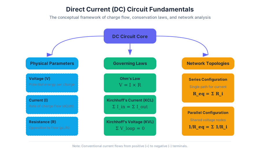
Direct Current (DC) circuits represent the foundational architecture of modern electronics. Unlike Alternating Current (AC), where the flow of charge periodically reverses direction, DC maintains a constant unidirectional flow. This stability makes it the preferred medium for digital logic, battery-powered systems, and the internal rails of almost every computing device in existence. To master DC circuits is to understand the fundamental interplay between energy, charge, and resistance.
The Foundations: Charge, Current, and Potential
Before diving into specific laws, we must establish the physical quantities that define a circuit. A circuit is essentially a closed loop through which charge ($Q$) flows. This flow is driven by a potential difference ($V$), often provided by a battery or power supply, which acts as a "pump" for electrons.
| Parameter | Symbol | Unit | Physical Interpretation |
|---|---|---|---|
| Voltage | $V$ | Volts (V) | The electrical potential energy per unit charge. |
| Current | $I$ | Amperes (A) | The rate of flow of electric charge ($I = dQ/dt$). |
| Resistance | $R$ | Ohms ($\Omega$) | The opposition to the flow of electric current. |
| Conductance | $G$ | Siemens (S) | The ease with which current flows ($G = 1/R$). |
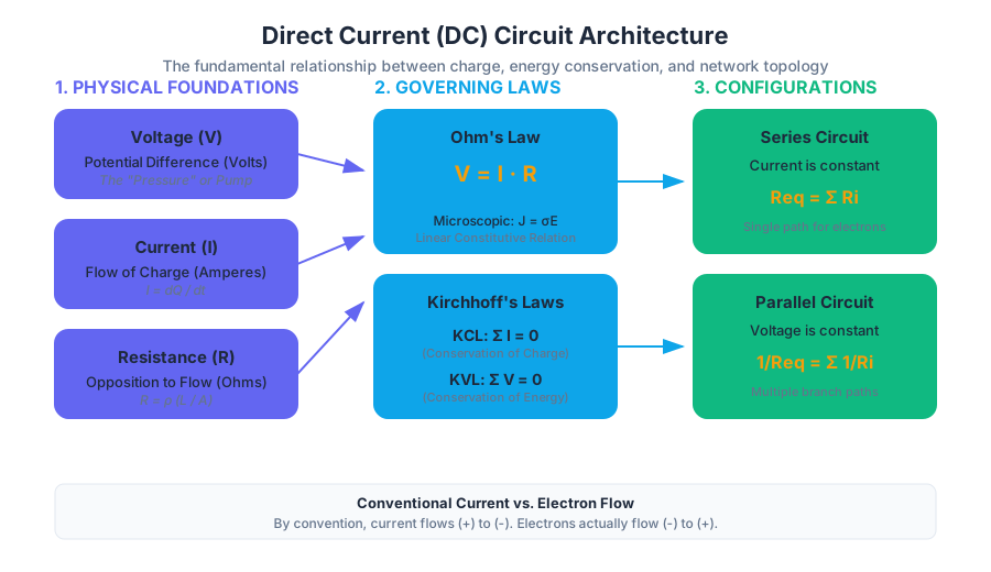
The Principle of Conventional Current: By historical convention (established by Benjamin Franklin), current is defined as the flow of positive charge. In reality, in metallic conductors, it is the negatively charged electrons that move. Thus, conventional current flows from the positive terminal to the negative terminal, while actual electron flow is the reverse.
Ohm’s Law: The Governing Equation
Ohm’s Law is the constitutive relation for a linear resistor. It states that the current through a conductor between two points is directly proportional to the voltage across the two points.
The Mathematical Formulation
The macroscopic form of Ohm's Law is: $$V = I \cdot R$$
However, for a deeper understanding, we look at the microscopic form, which relates the current density ($\mathbf{J}$) to the electric field ($\mathbf{E}$): $$\mathbf{J} = \sigma \mathbf{E}$$ where $\sigma$ is the conductivity of the material. This derivation highlights that resistance is not just a value on a component, but a property derived from the material's geometry and intrinsic resistivity ($\rho = 1/\sigma$).
Derivation of Resistance from Geometry
For a uniform conductor of length $L$ and cross-sectional area $A$: $$R = \rho \frac{L}{A}$$ This explains why longer wires have higher resistance and thicker wires have lower resistance—a crucial consideration in high-power DC distribution.
Kirchhoff’s Laws: The Conservation Principles
While Ohm's Law describes individual components, Kirchhoff’s Laws describe how those components interact within a network. They are the electrical equivalents of the conservation of charge and the conservation of energy.
Kirchhoff’s Current Law (KCL)
Theorem: The algebraic sum of currents entering a node (or a closed boundary) is zero. $$\sum_{k=1}^{n} I_k = 0$$ KCL is a statement of the Conservation of Charge. Since charge cannot build up at a point in a steady-state DC circuit, every electron entering a junction must leave it.
Kirchhoff’s Voltage Law (KVL)
Theorem: The algebraic sum of all voltages around any closed loop in a circuit is zero. $$\sum_{k=1}^{n} V_k = 0$$ KVL is a statement of the Conservation of Energy. If a charge travels in a complete loop and returns to its starting point, it must have the same potential energy it started with.
Circuit Configurations: Series and Parallel
Analyzing complex circuits requires simplifying networks into "equivalent" resistances.
Series Configurations
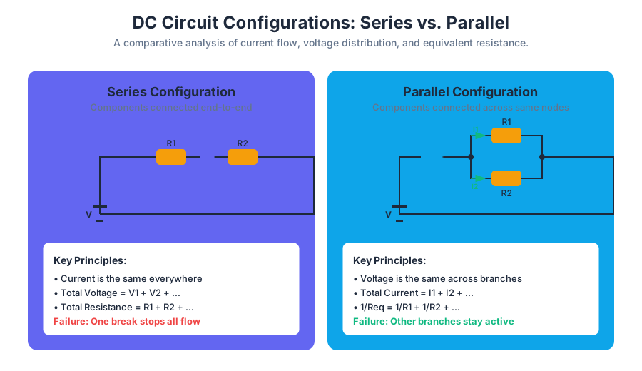
In a series circuit, components are connected end-to-end, forming a single path for current.
- Current is constant: $I_{total} = I_1 = I_2 = ... = I_n$.
- Voltages add up: $V_{total} = V_1 + V_2 + ... + V_n$.
- Equivalent Resistance: $R_{eq} = \sum R_i$.
Parallel Configurations
In a parallel circuit, components are connected across the same two nodes.
- Voltage is constant: $V_{total} = V_1 = V_2 = ... = V_n$.
- Currents add up: $I_{total} = I_1 + I_2 + ... + I_n$.
- Equivalent Resistance: $\frac{1}{R_{eq}} = \sum \frac{1}{R_i}$.
| Feature | Series Circuit | Parallel Circuit |
|---|---|---|
| Current Path | Single path | Multiple paths |
| Current Value | Same through all resistors | Divided among branches |
| Voltage Value | Divided across resistors | Same across all branches |
| Failure Result | One break stops all current | One break only affects that branch |
| Total Resistance | $R_{eq} >$ largest individual $R$ | $R_{eq} <$ smallest individual $R$ |
Electric Power and Joule Heating
Electric power ($P$) is the rate at which electrical energy is transferred by an electric circuit. In a resistor, this energy is converted into heat—a phenomenon known as Joule Heating.
The Power Formulas
Using Ohm's Law, we can derive three equivalent expressions for power:
- Primary: $P = V \cdot I$
- Current-centric: $P = I^2 \cdot R$ (Useful for series circuits)
- Voltage-centric: $P = \frac{V^2}{R}$ (Useful for parallel circuits)
Derivation of the $I^2R$ Relation
Work (W) = V \cdot Q
Power (P) = \frac{dW}{dt} = V \cdot \frac{dQ}{dt} = V \cdot I
Substitute V = IR:
P = (IR) \cdot I = I^2R
This relationship is critical in power distribution. To minimize power loss ($I^2R$) in transmission lines, engineers increase the voltage ($V$) to decrease the current ($I$) for a given power level.
Measurement: Ammeters and Voltmeters
To observe these theoretical values in the real world, we use measurement instruments. However, the act of measuring a circuit inevitably changes it.
Ammeters
An Ammeter measures current.
- Connection: Must be connected in series with the component.
- Ideal Characteristic: Zero internal resistance ($R_a = 0$).
- Real-world Pitfall: If an ammeter has significant resistance, it reduces the current it is trying to measure (Loading Effect).
Voltmeters
A Voltmeter measures potential difference.
- Connection: Must be connected in parallel with the component.
- Ideal Characteristic: Infinite internal resistance ($R_v = \infty$).
- Real-world Pitfall: If a voltmeter has low resistance, it draws current away from the circuit branch, lowering the measured voltage.
| Instrument | Ideal Resistance | Connection Type | Measured Quantity |
|---|---|---|---|
| Ammeter | $0$ | Series | Current (Flow) |
| Voltmeter | $\infty$ | Parallel | Potential (Pressure) |
| Ohmmeter | N/A | Parallel (Powered Off) | Resistance |
Advanced Analysis: The Loading Effect
When using a real voltmeter, we create a parallel path. If the circuit's Thevenin resistance is high, the voltmeter's resistance ($R_m$) significantly alters the total resistance.
Common Pitfalls in DC Analysis
- Short Circuits: Connecting a wire directly across a voltage source ($R \approx 0$). According to $I = V/R$, the current approaches infinity, leading to heat, fire, or component failure.
- Open Circuits: A break in the path ($R = \infty$). No current flows, but the full source voltage may still be present across the break.
- Grounding Misconceptions: "Ground" is simply a reference point (0V). It is not a magical sink for electrons, but a node we choose to call zero for the sake of calculation.
- Power Rating Overlook: Resistors are rated in Watts. Even if the resistance is correct, exceeding the power rating ($I^2R$) will cause the component to burn out.
Worked Example: Multi-Loop Analysis
Problem: A 12V battery is connected to a 4$\Omega$ resistor in series with a parallel combination of a 6$\Omega$ and a 12$\Omega$ resistor. Find the total current and the power dissipated by the 6$\Omega$ resistor.
Step 1: Find Equivalent Resistance ($R_{eq}$)
- Parallel part: $R_p = \frac{6 \cdot 12}{6 + 12} = \frac{72}{18} = 4\Omega$.
- Total resistance: $R_{total} = R_{series} + R_p = 4\Omega + 4\Omega = 8\Omega$.
Step 2: Find Total Current ($I_{total}$)
- $I_{total} = \frac{V}{R_{total}} = \frac{12V}{8\Omega} = 1.5A$.
Step 3: Find Voltage across the Parallel Branch ($V_p$)
- $V_p = I_{total} \cdot R_p = 1.5A \cdot 4\Omega = 6V$.
Step 4: Find Power in the 6$\Omega$ Resistor
- $P = \frac{V_p^2}{R} = \frac{6^2}{6} = \frac{36}{6} = 6W$.
Source Materials
Study High School Physics on Lykke
This course page is free to open: signed out, you can read its first two sections, and signing in, on any plan, opens the rest. The free Lykke Chrome extension syncs your own Canvas courses, so ChatGPT, Claude and Muse can answer from your classes and deadlines. It only reads Canvas.
Add the free extensionSign in to open every sectionAll sections of High School Physics · Browse more course pages