Geology

Introduction to Geology and the Scientific Method

Geology is the comprehensive study of the Earth, encompassing its composition, the physical and chemical processes that shape it, and the history of the planet and its life forms. Far from being a static catalog of rocks, modern geology is a dynamic, interdisciplinary field that integrates chemistry, physics, biology, and mathematics to understand the "Earth System." This section explores the foundational frameworks—the scientific method, specialized vocabulary, and the dual nature of physical and historical geology—that allow us to decode the 4.54 billion-year narrative of our planet.

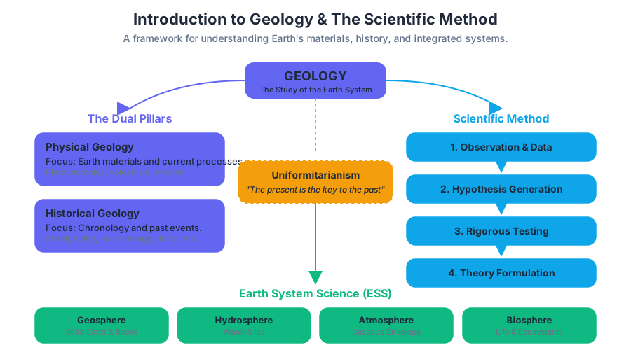
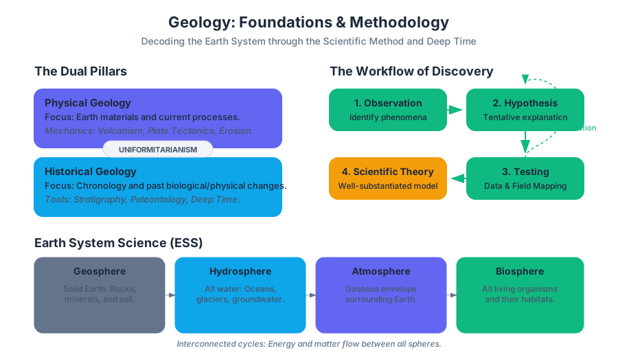
The Dual Pillars: Physical vs. Historical Geology

Geology is traditionally divided into two broad, overlapping sub-disciplines. While they share the same fundamental principles, their objectives and methodologies differ in scope and temporal focus.

Physical Geology

Physical Geology examines the materials composing Earth and seeks to understand the many processes that operate beneath and upon its surface. It focuses on the "mechanics" of the planetary engine, including volcanism, plate tectonics, rock formation, and erosion.

Historical Geology

Historical Geology aims to understand the origin of Earth and its development through time. It strives to establish a chronological arrangement of the vast physical and biological changes that have occurred in the geologic past. It relies heavily on stratigraphy (the study of rock layers) and paleontology (the study of fossils).

Feature	Physical Geology	Historical Geology
Primary Focus	Earth materials and current processes.	Chronology and past events.
Key Questions	How do mountains form? What is this mineral?	When did the Rockies rise? How did life evolve?
Core Concepts	Plate tectonics, Petrology, Mineralogy.	Stratigraphy, Paleontology, Deep Time.
Temporal Scale	Often focuses on the "instantaneous" or cyclical.	Focuses on linear time over billions of years.

The Scientific Method in Geoscience

Geology is an empirical science. Unlike "hard" sciences like physics where variables can be strictly controlled in a laboratory, geologists often deal with uncontrolled natural experiments that have run for millions of years. The Scientific Method in geology is an iterative process of observation, hypothesis generation, and rigorous testing.

The Workflow of Discovery

1. Observation: Identifying a phenomenon (e.g., "These two continents have matching fossil records").
2. Hypothesis: A tentative explanation (e.g., "The continents were once joined").
3. Testing and Data Collection: Gathering evidence through field mapping, isotopic dating, or seismic imaging.
4. Theory Building: If a hypothesis survives extensive scrutiny and competing explanations are eliminated, it may be elevated to a Theory (e.g., Plate Tectonics).

Definition: Scientific Theory A well-substantiated explanation of some aspect of the natural world that is acquired through the scientific method and repeatedly tested and confirmed through observation and experimentation. It is NOT a "hunch."

Abductive Reasoning: The Geologist's Tool

Because geologists cannot travel back in time, they often use abductive reasoning (inference to the best explanation). If a specific process (like a modern volcanic eruption) produces a specific result (a certain type of basalt), and we find that same result in ancient rocks, we infer the same process occurred in the past. This is the essence of Uniformitarianism: "The present is the key to the past."

Earth System Science (ESS)

Modern geology views the Earth not as a collection of isolated parts, but as a complex, integrated system. Earth System Science (ESS) studies the interactions between the "spheres" of our planet.

Sphere	Description	Geological Interaction
Geosphere (Lithosphere)	The solid Earth (rocks, minerals, soil).	Plate movements create habitats and influence climate.
Hydrosphere	All Earth's water (oceans, glaciers, groundwater).	Water is the primary agent of erosion and sediment transport.
Atmosphere	The gaseous envelope surrounding the planet.	Volcanic outgassing created the early atmosphere.
Biosphere	All living organisms.	Life (e.g., stromatolites) altered the atmosphere's oxygen levels.

Implementation Example: Radioactive Decay Modeling

To understand the age of the Earth, geologists use the physics of radioactive decay. The following Python snippet demonstrates how we calculate the remaining parent isotopes in a sample to determine its "geologic age."

import numpy as np
import matplotlib.pyplot as plt

def calculate_decay(initial_atoms, half_life, time_elapsed):
    """
    Calculates the number of remaining parent atoms using the decay constant.
    Formula: N(t) = N0 * e^(-lambda * t)
    where lambda = ln(2) / half_life
    """
    decay_constant = np.log(2) / half_life
    remaining_atoms = initial_atoms * np.exp(-decay_constant * time_elapsed)
    return remaining_atoms

# Parameters for Uranium-238 to Lead-206 decay
N0 = 1000000  # Initial atoms
T_HALF = 4.47e9 # Half-life in years (4.47 billion years)
time_steps = np.linspace(0, 15e9, 100) # 0 to 15 billion years

remaining = calculate_decay(N0, T_HALF, time_steps)

plt.figure(figsize=(10, 5))
plt.plot(time_steps / 1e9, remaining, label='Parent Isotopes (U-238)')
plt.plot(time_steps / 1e9, N0 - remaining, label='Daughter Isotopes (Pb-206)', linestyle='--')
plt.title("Radioactive Decay Curve in Geochronology")
plt.xlabel("Time (Billions of Years)")
plt.ylabel("Number of Atoms")
plt.legend()
plt.grid(True)
plt.show()

Geological Vocabulary and Communication

Precision in language is vital in geology because terms often carry specific genetic implications (how something formed). For example, calling a rock "granite" implies a specific mineralogy and an intrusive igneous origin.

The Taxonomy of Earth Materials

• Minerals: Naturally occurring, inorganic solids with a definite chemical composition and ordered internal structure.
• Rocks: Aggregates of one or more minerals.
  • Igneous: Formed from cooling magma/lava.
  • Sedimentary: Formed from lithified sediment or chemical precipitation.
  • Metamorphic: Formed by altering existing rocks via heat and pressure.

Measurement and Observation

Geologists use specific tools to quantify the subsurface. Structural Geology involves measuring the orientation of rock layers using "Strike and Dip."

\text{Airy Isostasy Equation:} \\
h_r = \frac{\rho_c}{\rho_m - \rho_c} \cdot h_s \\
\text{Where: } \\
h_r = \text{thickness of the mountain root} \\
h_s = \text{height of the mountain above sea level} \\
\rho_c = \text{density of the crust} \\
\rho_m = \text{density of the mantle}

Plate Tectonics: The Unifying Theory

If the scientific method is the "how," Plate Tectonics is the "why" of geology. It provides a framework that explains earthquakes, volcanoes, mountain building, and the distribution of fossils.

1. The Lithosphere: The rigid outer shell of the Earth, broken into plates.
2. The Asthenosphere: The ductile layer of the mantle upon which plates "float."
3. Plate Boundaries:
   • Divergent: Plates move apart (e.g., Mid-Atlantic Ridge).
   • Convergent: Plates collide (e.g., The Himalayas).
   • Transform: Plates slide past each other (e.g., San Andreas Fault).

Boundary Type	Motion	Resulting Feature	Example
Divergent	Spreading	Oceanic Ridges / Rifts	East African Rift
Convergent (O-C)	Subduction	Volcanic Arcs / Trenches	Andes Mountains
Convergent (C-C)	Collision	Fold-Thrust Mountains	Alps
Transform	Lateral Slip	Fault Zones	North Anatolian Fault

Deep Time and the Geologic Time Scale

One of the most difficult concepts for the human mind to grasp is Deep Time. While human history spans thousands of years, geologic history spans billions.

The Eon-Era-Period Hierarchy

The Geologic Time Scale is a system of chronological dating that relates geological strata to time. It is divided into:

• Eons: The largest division (e.g., Phanerozoic).
• Eras: Subdivisions of eons (e.g., Mesozoic - "Age of Dinosaurs").
• Periods: Subdivisions of eras (e.g., Jurassic).
• Epochs: Subdivisions of periods (e.g., Holocene).

Practical Data Interaction

Geologists often query large datasets to find patterns in seismic activity or resource distribution. Below is a conceptual SQL query for an earthquake database.

-- Querying the USGS Earthquake Database for high-magnitude events 
-- near a specific tectonic boundary (Transform)
SELECT 
    event_id, 
    magnitude, 
    depth_km, 
    latitude, 
    longitude,
    timestamp
FROM 
    global_seismicity
WHERE 
    magnitude > 6.5 
    AND depth_km < 30 -- Shallow earthquakes are more destructive
    AND region = 'San Andreas Fault System'
ORDER BY 
    timestamp DESC;

Resource Accessibility and Social Impact

Geology is not purely academic; it is the foundation of the global economy. The study of Energy and Mineral Resources dictates where we get the materials for modern life.

• Critical Minerals: Elements like Lithium and Cobalt, essential for green energy, are found in specific geological settings (pegmatites or brine deposits).
• Water Resources: Hydrogeology studies the movement of water through aquifers, a critical skill as climate change impacts water security.
• Geohazards: Understanding the recurrence intervals of floods, landslides, and eruptions is essential for urban planning and disaster mitigation.

Common Pitfalls and Misconceptions

1. "Rocks are permanent": In reality, the Rock Cycle ensures that every rock is eventually recycled through subduction or erosion.
2. "The Earth is solid": While the mantle is solid rock, it behaves as a high-viscosity fluid over geologic timescales (mantle convection).
3. "Geology is just naming things": Modern geology is highly quantitative. It involves complex fluid dynamics, thermodynamics, and chemical modeling.

Summary of the Geological Workflow

To conclude, the study of geology follows a rigorous pipeline:

1. Field Observation: Mapping and measuring structures in the crust.
2. Sample Analysis: Using tools like the Petrographic Microscope to identify minerals and textures.
3. Deduction: Using the laws of stratigraphy and physics to reconstruct the sequence of events.
4. Synthesis: Integrating local findings into the global Plate Tectonics model.

Further Reading and References

• Johnson, C., et al. (2019). An Introduction to Geology.
• Waldron, J.W.F., & Snyder, M.C. (2020). Geological Structures: A Practical Introduction.
• Earle, S. (2015). Physical Geology.
• Ruppert, S., et al. Introduction to Historical Geology.

Minerals: The Building Blocks of Earth

Minerals are the fundamental units of the geosphere, representing the naturally occurring, inorganic solids that constitute the Earth's crust and mantle. To a geologist, a mineral is not merely a "rock component" but a highly ordered chemical system. Every mineral possesses a specific chemical composition and a characteristic crystalline structure, which dictates its physical properties—from the hardness of a diamond to the perfect cleavage of mica.

Understanding minerals requires an interdisciplinary approach, blending solid-state chemistry, geometry (crystallography), and classical physics (optics). This article provides a deep dive into the mechanics of mineral formation, the structural hierarchy of silicates, and the analytical methods used to identify these materials at the atomic and macroscopic scales.

Mineral Chemistry: The Laws of Atomic Architecture

At its core, mineralogy is the study of how atoms pack together in the solid state. Unlike liquids or gases, minerals are defined by long-range periodic order. The chemical identity of a mineral is determined by the ions present and the nature of the bonds between them.

The Nature of Bonding

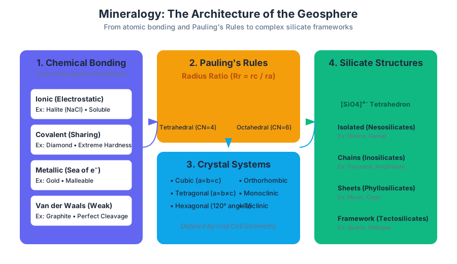
Most minerals are held together by a combination of ionic and covalent bonds. However, the physical behavior of a mineral is often dictated by its weakest bond. For instance, graphite and diamond are both pure carbon (polymorphs), but diamond’s three-dimensional covalent network makes it the hardest known natural substance, while graphite’s weak Van der Waals forces between sheets allow it to be used as a lubricant.

Bond Type	Mechanism	Mineral Example	Physical Property Impact
Ionic	Electrostatic attraction between oppositely charged ions	Halite (NaCl)	High solubility, moderate hardness
Covalent	Sharing of electron pairs between atoms	Diamond (C)	Extreme hardness, high melting point
Metallic	Delocalized "sea" of electrons	Native Gold (Au)	Malleability, high conductivity
Van der Waals	Weak dipole-dipole interactions	Graphite (C), Talc	Perfect cleavage, "greasy" feel

Pauling’s Rules and Coordination

To predict how minerals form, we use Pauling’s Rules, which govern the stability of ionic crystals. The most critical is the Radius Ratio Rule, which determines the coordination number (CN)—the number of anions surrounding a central cation.

The Radius Ratio ($R_r$): Defined as the ratio of the radius of the cation ($r_c$) to the radius of the anion ($r_a$). $$R_r = \frac{r_{cation}}{r_{anion}}$$

Worked Example: Predicting Coordination

If we have a Magnesium ion ($Mg^{2+}$, radius $\approx 0.72 \text{ \AA}$) and an Oxygen ion ($O^{2-}$, radius $\approx 1.40 \text{ \AA}$): $$R_r = \frac{0.72}{1.40} \approx 0.514$$ Looking at the coordination table, a ratio of 0.514 falls into the range of Octahedral Coordination (CN=6). This explains why $Mg$ typically sits in octahedral sites within silicate structures like Olivine.

# Python implementation to predict Coordination Number based on Pauling's Rules
def get_coordination_geometry(r_cation, r_anion):
    ratio = r_cation / r_anion
    
    limits = [
        (0.155, 0.225, 3, "Trigonal"),
        (0.225, 0.414, 4, "Tetrahedral"),
        (0.414, 0.732, 6, "Octahedral"),
        (0.732, 1.000, 8, "Cubic"),
        (1.000, float('inf'), 12, "Dodecahedral")
    ]
    
    for low, high, cn, geometry in limits:
        if low <= ratio < high:
            return {"CN": cn, "Geometry": geometry, "Ratio": round(ratio, 3)}
    return "Unknown/Unstable"

# Example: Silicon in Oxygen framework
# Si4+ ~ 0.26 A, O2- ~ 1.35 A
print(get_coordination_geometry(0.26, 1.35))
# Output: {'CN': 4, 'Geometry': 'Tetrahedral', 'Ratio': 0.193}

Crystallography: Symmetry and the Lattice

Crystallography is the mathematical description of the internal order of minerals. A crystal is formed by the repetition of a unit cell—the smallest repeating unit that retains the full symmetry of the crystal.

The 7 Crystal Systems

All minerals fall into one of seven systems based on the geometry of their unit cell (lengths of axes $a, b, c$ and angles $\alpha, \beta, \gamma$).

System	Axial Relationships	Angles	Examples
Cubic (Isometric)	$a = b = c$	$\alpha = \beta = \gamma = 90^\circ$	Garnet, Pyrite, Halite
Tetragonal	$a = b \neq c$	$\alpha = \beta = \gamma = 90^\circ$	Zircon, Rutile
Orthorhombic	$a \neq b \neq c$	$\alpha = \beta = \gamma = 90^\circ$	Olivine, Topaz
Hexagonal	$a_1 = a_2 = a_3 \neq c$	$\alpha = \beta = 90^\circ, \gamma = 120^\circ$	Quartz, Apatite
Monoclinic	$a \neq b \neq c$	$\alpha = \gamma = 90^\circ, \beta \neq 90^\circ$	Orthoclase, Gypsum
Triclinic	$a \neq b \neq c$	$\alpha \neq \beta \neq \gamma \neq 90^\circ$	Plagioclase, Albite

Miller Indices

To describe specific planes of atoms within a crystal, we use Miller Indices $(hkl)$. These are the reciprocals of the intercepts that a plane makes with the crystallographic axes.

\text{Step 1: Identify intercepts on axes } a, b, c. \text{ (e.g., 1, 2, } \infty)
\text{Step 2: Take reciprocals: } \frac{1}{1}, \frac{1}{2}, \frac{1}{\infty} \rightarrow 1, 0.5, 0
\text{Step 3: Clear fractions to find smallest integers: } (2 1 0)

Silicate Minerals: The Framework of the Crust

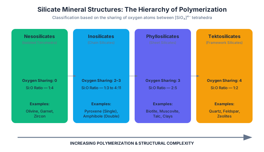
Over 90% of the Earth's crust is composed of silicates. The fundamental building block of all silicates is the Silicon-Oxygen Tetrahedron $[SiO_4]^{4-}$. The diversity of silicate minerals arises from polymerization—the sharing of oxygen atoms between tetrahedra.

The Silicate Classification Hierarchy

Silicates are classified by how their tetrahedra are linked. This structure directly influences the mineral's cleavage and stability.

1. Nesosilicates (Island): Isolated tetrahedra linked by cations (e.g., Olivine).
2. Sorosilicates (Double): Two tetrahedra sharing one oxygen.
3. Cyclosilicates (Ring): Tetrahedra linked in rings (e.g., Beryl/Emerald).
4. Inosilicates (Chain): Single chains (Pyroxenes) or double chains (Amphiboles).
5. Phyllosilicates (Sheet): Tetrahedra sharing three oxygens to form 2D sheets (e.g., Micas, Clays).
6. Tectosilicates (Framework): Every oxygen is shared, forming a 3D network (e.g., Quartz, Feldspar).

Silicate Group	O:Si Ratio	Structure	Cleavage Pattern
Nesosilicates	4:1	Isolated	None/Conchoidal
Inosilicates (Single)	3:1	Single Chain	2 planes at ~90°
Inosilicates (Double)	2.75:1	Double Chain	2 planes at 56°/124°
Phyllosilicates	2.5:1	Sheet	1 perfect basal plane
Tectosilicates	2:1	3D Framework	Complex or None

Optical Mineralogy: Light as a Diagnostic Tool

When light enters a non-opaque mineral, it interacts with the crystal lattice in ways that allow for precise identification using a petrographic microscope.

Isotropic vs. Anisotropic

• Isotropic minerals (Cubic system): Light travels at the same speed in all directions. They appear dark under Cross-Polarized Light (XPL).
• Anisotropic minerals (All other systems): Light is split into two rays traveling at different velocities. This phenomenon is known as Birefringence.

The Michel-Lévy Chart and Retardation

The difference in speed between the "fast" and "slow" rays results in a phase shift called retardation ($\Delta$). When the rays recombine, they produce interference colors.

Formula for Birefringence ($\delta$): $$\delta = \frac{\Delta}{d}$$ Where $d$ is the thickness of the thin section (standardized at 30 microns).

Common Pitfalls in Optical Identification

A common mistake for students is confusing extinction with isotropy. An anisotropic mineral will go dark (extinguish) every 90 degrees of rotation in XPL, whereas an isotropic mineral remains dark throughout the full 360-degree rotation.

Gemstone Identification: Beyond the Loupe

Gemology is the applied science of mineralogy focused on "precious" specimens. Identification relies on non-destructive testing to differentiate natural stones from synthetics and "simulants" (imitations).

Specific Gravity (SG)

SG is a measure of density relative to water. It is a critical diagnostic because chemical composition is fixed. $$SG = \frac{W_{air}}{W_{air} - W_{water}}$$

Refractive Index (RI)

Using a refractometer, gemologists measure how much light bends as it enters the stone. Since many gems are anisotropic, they will show two RIs (birefringence). For example:

• Diamond: RI = 2.417 (Singly refractive)
• Ruby/Sapphire: RI = 1.762 – 1.770 (Doubly refractive, $\delta = 0.008$)

Spectroscopic Analysis

Advanced identification uses Raman Spectroscopy or FTIR. These tools detect the vibrational modes of the crystal lattice, allowing gemologists to identify heat treatments or polymer injections in emeralds.

# Example CLI interaction with a hypothetical Mineral Analysis Database (MinDB)
# Querying for diagnostic properties of a suspected Corundum sample

$ mindb query --name "Corundum" --properties "RI, Hardness, System"

[Results]
Mineral: Corundum (Al2O3)
Crystal System: Hexagonal (Trigonal)
Hardness (Mohs): 9.0
Refractive Index: 1.762 - 1.770
Birefringence: 0.008 (Uniaxial Negative)
Common Varieties: Ruby (Cr-bearing), Sapphire (Fe/Ti-bearing)

$ mindb compare --sample_ri 1.72 --sample_sg 3.60
[Match Found]
Mineral: Spinel (MgAl2O4)
Confidence: 94%
Note: Often confused with Ruby; check for lack of pleochroism.

Practical Identification Pipeline

When a geologist encounters an unknown mineral in the field, they follow a systematic "elimination" pipeline:

1. Luster: Is it metallic or non-metallic?
2. Hardness: Can it be scratched by a copper penny (3.5), a glass plate (5.5), or a steel file (6.5)?
3. Cleavage/Fracture: Does it break along flat planes (cleavage) or irregular surfaces (fracture)?
4. Streak: What is the color of the mineral in powdered form? (Crucial for metallic minerals).
5. Specific Gravity: Does it feel "heavy" for its size (e.g., Galena or Barite)?

Summary of Mineral Groups

While silicates dominate, other groups are economically and geologically vital:

Group	Anion / Complex	Examples	Importance
Native Elements	Single element	Gold, Diamond, Sulfur	Rare, economically valuable
Oxides	$O^{2-}$	Hematite, Magnetite	Primary iron ores
Sulfides	$S^{2-}$	Pyrite, Galena	Metal ores (Pb, Zn, Cu)
Carbonates	$[CO_3]^{2-}$	Calcite, Dolomite	Carbon cycle, limestone
Halides	$Cl^-, F^-$	Halite, Fluorite	Industrial salts, flux
Sulfates	$[SO_4]^{2-}$	Gypsum, Barite	Evaporites, construction

Igneous Processes and Volcanism

Igneous processes represent the primary engine of Earth’s crustal evolution. Derived from the Latin ignis (fire), igneous rocks are the products of the cooling and solidification of molten rock. This cycle begins deep within the mantle or lower crust where phase transitions turn solid rock into magma, and ends either deep underground as plutons or at the surface as lava and tephra. Understanding these processes is not merely an exercise in classification; it is the study of the thermal and chemical differentiation of our planet.

The Physics and Chemistry of Melt

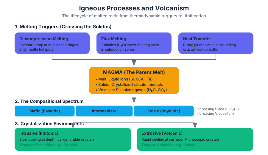
To understand igneous rocks, one must first understand the state of the parent material. Magma is a complex, high-temperature solution consisting of three components:

1. Melt: The liquid portion, composed primarily of mobile ions (Si, O, Al, Ca, Fe, Mg, Na, K).
2. Solids: Any silicate minerals that have already crystallized from the melt.
3. Volatiles: Dissolved gases, primarily $H_2O$, $CO_2$, and $SO_2$, which remain in solution due to high confining pressure.

The Thermodynamics of Melting

Contrary to popular belief, the Earth’s mantle is not a sea of liquid magma; it is a plastic solid. Magma only forms under specific thermodynamic "triggers" that cross the solidus (the temperature at which a rock begins to melt).

The Solidus-Liquidus Gap: The Solidus is the locus of points in P-T space below which a substance is completely solid. The Liquidus is the boundary above which it is completely liquid. Between them lies a "mush zone" of partial melting.

There are three primary mechanisms for generating melt:

• Decompression Melting: Reducing pressure without losing heat. This occurs at mid-ocean ridges and hotspots.
• Flux Melting: The introduction of volatiles (like water) into the hot mantle, which lowers the melting temperature. This is the primary driver of subduction zone volcanism.
• Heat Transfer: Direct heating of crustal rocks by rising mantle plumes.

Magma Compositional Spectrum

The chemistry of magma is defined by its Silica ($SiO_2$) content, which dictates its viscosity, density, and eruptive style.

Magma Type	Silica Content ($SiO_2$)	Temperature (°C)	Viscosity	Gas Content	Resulting Rock (Extrusive)
Felsic (Rhyolitic)	>65%	600–800	Very High	High	Rhyolite
Intermediate (Andesitic)	55–65%	800–1000	Intermediate	Intermediate	Andesite
Mafic (Basaltic)	45–55%	1000–1200	Low	Low	Basalt
Ultramafic	<45%	>1200	Very Low	Very Low	Komatiite (rare)

Petrology: The Science of Rock Origins

Petrology is the branch of geology that studies the origin, composition, and structure of rocks. In the igneous context, we differentiate rocks based on their texture (cooling history) and mineralogy (chemical composition).

Intrusive vs. Extrusive

The most fundamental division in petrology is based on the environment of crystallization.

1. Intrusive (Plutonic): Magma that crystallizes at depth. Because the surrounding "country rock" acts as an insulator, heat loss is extremely slow. This allows ions to migrate to existing crystal seeds, resulting in large, visible crystals (Phaneritic texture).
2. Extrusive (Volcanic): Magma that reaches the surface (lava). Rapid cooling against the air or water prevents large crystal growth, resulting in a fine-grained (Aphanitic) or even glassy (Vitreous) texture.

Texture as a Diagnostic Tool

Texture provides a "fossilized" record of the cooling rate.

Texture	Cooling Rate	Description	Typical Environment
Phaneritic	Slow	Coarse-grained; crystals visible to the naked eye.	Deep Plutons
Aphanitic	Fast	Fine-grained; crystals require magnification.	Lava Flows
Porphyritic	Bimodal	Large crystals (phenocrysts) in a fine matrix.	Two-stage cooling
Vitreous	Instantaneous	Glassy; no crystalline structure.	Obsidian flows
Vesicular	Rapid	Pitted with gas bubbles (vesicles).	Top of lava flows
Pyroclastic	Explosive	Fragmented rock, ash, and glass shards.	Volcanic eruptions

Bowen’s Reaction Series: The Chemical Blueprint

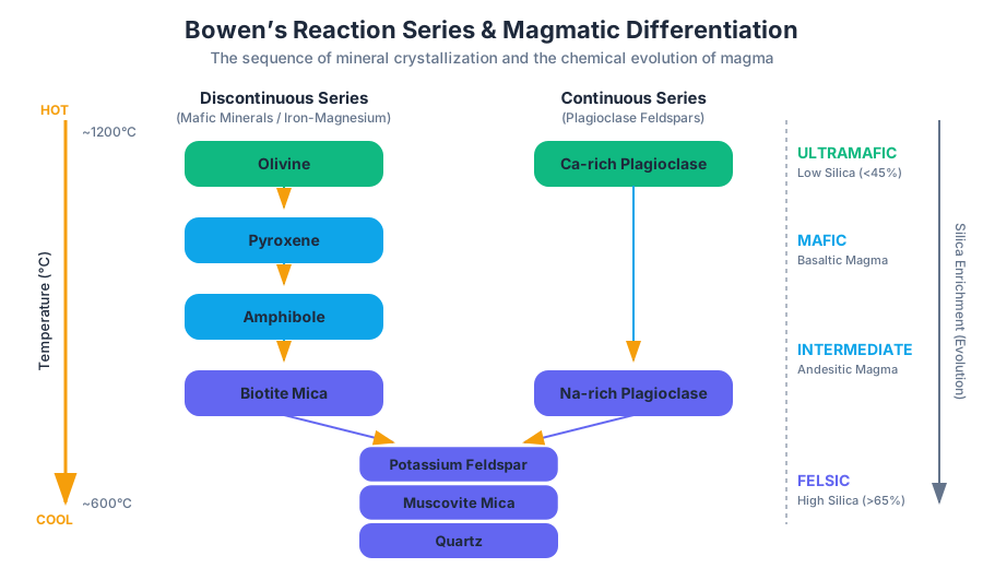
In the early 20th century, N.L. Bowen discovered that minerals do not crystallize simultaneously. Instead, they follow a predictable sequence as temperature drops. This is the Bowen’s Reaction Series, which explains why certain minerals (like quartz and olivine) are rarely found in the same rock.

The Discontinuous Series

As the melt cools, the first mineral to form is Olivine. As the temperature drops further, the olivine reacts with the remaining melt to form Pyroxene, then Amphibole, and finally Biotite Mica. Each step represents a fundamental change in the silicate structure, moving from isolated tetrahedra to single chains, double chains, and finally sheets.

The Continuous Series

Simultaneously, Plagioclase Feldspar crystallizes. It begins as calcium-rich (Anorthite) and continuously exchanges Ca for Na as the temperature decreases, ending as sodium-rich (Albite).

Magmatic Differentiation

If crystals are removed from the melt (e.g., by gravity settling), the remaining liquid becomes "evolved"—it is depleted in Mg and Fe and enriched in Si, Na, and K. This process allows a single parent mafic magma to produce a variety of intermediate and felsic daughter rocks.

# A simplified simulation of Magmatic Differentiation
# Tracking the enrichment of Silica as Mafic minerals crystallize

import numpy as np

def simulate_crystallization(initial_si, cooling_steps):
    melt_composition = {"SiO2": initial_si, "MgFe": 100 - initial_si}
    history = []

    for step in range(cooling_steps):
        # Mafic minerals (MgFe rich) crystallize first, 
        # removing more MgFe than SiO2 from the melt.
        crystallization_rate = 0.05  # 5% of melt crystallizes per step
        mafic_fraction_in_crystal = 0.8 # Crystals are 80% MgFe
        
        crystals_mass = melt_composition["MgFe"] * crystallization_rate
        
        # Update melt: remove mass from MgFe and SiO2
        melt_composition["MgFe"] -= crystals_mass * mafic_fraction_in_crystal
        melt_composition["SiO2"] -= crystals_mass * (1 - mafic_fraction_in_crystal)
        
        # Recalculate percentages
        total = melt_composition["MgFe"] + melt_composition["SiO2"]
        si_percent = (melt_composition["SiO2"] / total) * 100
        history.append(round(si_percent, 2))
        
    return history

# Starting with a Basaltic melt (~50% SiO2)
evolution = simulate_crystallization(50.0, 10)
print(f"Melt Evolution (SiO2 %): {evolution}")
# Output shows the melt becoming increasingly Felsic (Rhyolitic)

Volcanism: The Surface Expression

When magma breaches the surface, it becomes lava. The style of the resulting eruption is governed by the Gas-Viscosity Paradox: high-viscosity melts trap gas more effectively, leading to explosive pressure build-ups.

Volcano Morphologies

The physical shape of a volcano is a direct function of the rheology of its lava.

Volcano Type	Magma Type	Shape	Eruptive Style
Shield	Mafic	Broad, low-profile (e.g., Mauna Loa)	Effusive (Lava flows)
Composite (Stratovolcano)	Intermediate/Felsic	Tall, steep, conical (e.g., Mt. St. Helens)	Explosive
Cinder Cone	Mafic/Intermediate	Small, steep, made of scoria	Sputtering (Strombolian)
Caldera	Felsic	Large depression from collapsed chamber	Catastrophic collapse

Volcanic Hazards

Volcanism poses diverse threats to human infrastructure and life.

1. Pyroclastic Density Currents (PDCs): Gravity-driven clouds of hot gas and ash. They can travel at speeds >100 km/h and temperatures >500°C.
2. Lahars: Volcanic mudflows triggered by the melting of snow/ice or heavy rain on loose ash. They have the consistency of wet concrete.
3. Tephra Fall: Ash and lapilli can collapse roofs, destroy aircraft engines, and cause respiratory failure.
4. Lava Flows: While rarely life-threatening due to slow speeds, they are unstoppable and destroy all property in their path.

The VEI Scale: The Volcanic Explosivity Index (VEI) is a relative measure of the explosiveness of volcanic eruptions. It is logarithmic, ranging from 0 (non-explosive) to 8 (mega-colossal).

\text{The Clausius-Clapeyron Relation for Decompression Melting:} \\
\frac{dP}{dT} = \frac{L}{T \Delta V} \\
\text{Where:} \\
P = \text{Pressure} \\
T = \text{Temperature} \\
L = \text{Latent heat of fusion} \\
\Delta V = \text{Change in specific volume during melting} \\
\text{Insight: Since rocks expand when they melt (positive } \Delta V \text{),} \\
\text{decreasing pressure (negative } dP \text{) lowers the melting temperature.}

Worked Example: Calculating Crystal Settling (Stokes' Law)

In a cooling magma chamber, how fast does an olivine crystal sink? This determines the degree of magmatic differentiation.

Given:

• Crystal radius ($r$): 0.002 m (2mm)
• Density of Olivine ($\rho_s$): 3300 $kg/m^3$
• Density of Basaltic melt ($\rho_f$): 2700 $kg/m^3$
• Viscosity of melt ($\eta$): 100 $Pa \cdot s$
• Gravity ($g$): 9.8 $m/s^2$

Formula (Stokes' Law): $$v = \frac{2}{9} \frac{(\rho_s - \rho_f) g r^2}{\eta}$$

Calculation:

1. $\Delta \rho = 3300 - 2700 = 600$
2. $r^2 = 0.000004$
3. $v = (2/9) * (600 * 9.8 * 0.000004) / 100$
4. $v \approx 0.22 * (0.02352) / 100$
5. $v \approx 0.000052$ m/s $\approx$ 4.5 meters per day.

Conclusion: In a large magma chamber (kilometers deep), olivine crystals can settle to the floor over decades, creating a "cumulate" layer and changing the chemistry of the remaining melt.

Common Pitfalls in Igneous Geology

• "Magma is just melted rock": While true, the process of melting is usually partial. A rock rarely melts 100%; instead, the silica-rich components melt first, leaving behind a "restite" of mafic minerals.
• Confusing Viscosity with Density: Felsic magma is less dense than mafic magma (it rises), but it is more viscous (it flows poorly). Students often assume "thicker" means "heavier."
• Obsidian is Felsic: Despite its dark color (caused by trace iron), obsidian is almost always rhyolitic (felsic). Color is a poor proxy for composition in glasses.

# Example: Accessing USGS Volcano Hazards Program API for Real-time Monitoring
# This script fetches the current alert level for a specific volcano (e.g., Kilauea)

VOLCANO_ID="Kilauea"
API_URL="https://volcanoes.usgs.gov/hans-public/api/v1/status"

# Fetch status and filter for the specific volcano
curl -s $API_URL | jq '.features[] | select(.properties.volcano_name == "'$VOLCANO_ID'") | {name: .properties.volcano_name, alert_level: .properties.alert_level, color: .properties.v_color_code}'

Weathering, Sediments, and Sedimentary Rocks: The Earth's Surface Archive

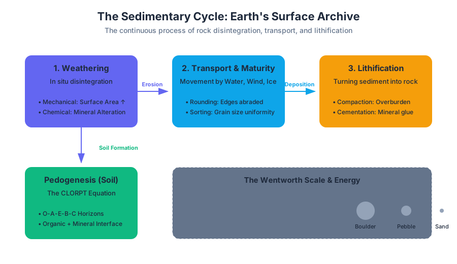
The Earth’s surface is a dynamic interface where the lithosphere, hydrosphere, atmosphere, and biosphere converge. This intersection facilitates the sedimentary cycle, a continuous process of rock degradation, transport, and reconstruction. Unlike igneous and metamorphic rocks, which often originate in high-pressure, high-temperature environments deep within the crust, sedimentary rocks are the primary records of Earth's surface history. They archive the evolution of life (fossils), fluctuations in ancient climates, and the migration of tectonic plates.

1. Weathering: The Engine of Disintegration

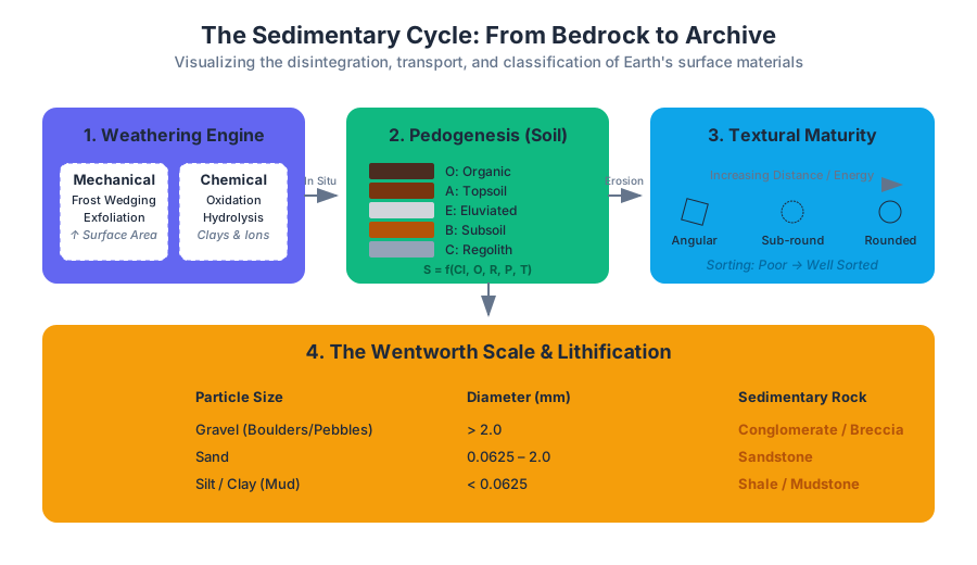
Weathering is the in situ physical disintegration and chemical decomposition of rocks. It is distinct from erosion, which involves the transport of the resulting debris. Weathering acts as the precursor to the sedimentary cycle by reducing solid bedrock into transportable particles and dissolved ions.

1.1 Mechanical Weathering

Mechanical (or physical) weathering involves the physical breakage of rock into smaller fragments without changing the mineral chemistry. This process is critical because it exponentially increases the surface area available for chemical attack.

Mechanism	Description	Primary Environment
Frost Wedging	Water enters cracks, freezes, expands by ~9%, and exerts outward pressure.	Alpine/Sub-polar
Exfoliation	Pressure release (unloading) causes plutonic rocks to expand and peel in sheets.	High-relief granitic terrains
Thermal Expansion	Differential expansion of minerals due to extreme diurnal temperature swings.	Arid Deserts
Biogenic Activity	Root wedging and animal burrowing physically displace rock material.	Vegetated regions

1.2 Chemical Weathering

Chemical weathering involves the transformation of original minerals into new, stable phases (usually clays) and dissolved ions. This process is governed by the principles of chemical equilibrium; minerals formed at high temperatures (e.g., Olivine) are most unstable at the Earth's surface.

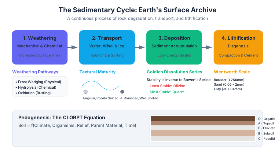
Goldich Dissolution Series: A conceptual model stating that the order of mineral weathering is the inverse of Bowen's Reaction Series. Olivine weathers most rapidly, while Quartz is the most resistant.

The primary chemical pathways include:

1. Oxidation: Reaction with oxygen (e.g., $4Fe^{2+} + 3O_2 \rightarrow 2Fe_2O_3$, forming hematite/rust).
2. Hydrolysis: Reaction with $H^+$ and $OH^-$ ions in water, typically converting silicates to clay minerals.
3. Carbonation: Dissolution by carbonic acid ($H_2CO_3$), formed when $CO_2$ dissolves in rainwater.

/* 
 * Low-level Simulation: Mechanical Weathering Surface Area Increase
 * This C snippet calculates the exponential increase in surface area 
 * as a cubic rock is subdivided into smaller units.
 */

#include <stdio.h>
#include <math.h>

typedef struct {
    double side_length; // in meters
    long long count;
} RockMass;

void calculate_surface_area(RockMass rm) {
    double total_area = 6 * pow(rm.side_length, 2) * rm.count;
    double total_volume = pow(rm.side_length, 3) * rm.count;
    printf("Units: %lld | Side: %.6f m | Area: %.2f m^2 | Vol: %.2f m^3\n", 
            rm.count, rm.side_length, total_area, total_volume);
}

int main() {
    RockMass rock = {1.0, 1}; // Start with a 1m cube
    printf("Simulating physical fragmentation (halving side length per step):\n");
    
    for (int i = 0; i < 10; i++) {
        calculate_surface_area(rock);
        rock.side_length /= 2.0;
        rock.count *= 8; // Each cube splits into 8 smaller cubes
    }
    return 0;
}

2. Pedogenesis: The Formation of Soil

Soil is the bridge between the inorganic and organic worlds. It is defined as a combination of mineral matter, organic matter (humus), water, and air. Pedogenesis (soil formation) is controlled by the CLORPT equation:

$$S = f(Cl, O, R, P, T)$$

Where:

• Cl: Climate (Temperature and precipitation)
• O: Organisms (Biological activity)
• R: Relief (Topography and slope)
• P: Parent Material (The source rock)
• T: Time (Duration of weathering)

2.1 Soil Horizons

As soil matures, it develops distinct layers called horizons.

Horizon	Name	Characteristics
O	Organic	Fresh and decaying organic matter (humus).
A	Topsoil	Mineral matter mixed with humus; high biological activity.
E	Eluviated	Zone of leaching; light-colored, depleted of clay and iron.
B	Subsoil	Zone of accumulation (illuviation) of minerals from above.
C	Regolith	Partially altered parent material.
R	Bedrock	Unweathered source rock.

3. Sediment Transport and Deposition

Once rock is weathered, it becomes sediment. The transport of this sediment is a function of the medium's energy (water, wind, or ice).

3.1 Textural Maturity

As sediment is transported further from its source, it undergoes predictable changes:

• Rounding: Angular edges are abraded; grains become spherical.
• Sorting: The range of grain sizes narrows. High-energy environments (e.g., mountain streams) have poor sorting; low-energy environments (e.g., deep lakes) have high sorting.
• Mineral Maturity: Unstable minerals (feldspars, micas) disappear, leaving only resistant minerals like quartz.

3.2 The Wentworth Scale

Geologists use the Wentworth Scale to classify sediment by diameter ($d$):

Particle	Size Range ($mm$)	Typical Rock Equivalent
Boulder	$> 256$	Conglomerate / Breccia
Cobble	$64 - 256$	Conglomerate / Breccia
Pebble	$2 - 64$	Conglomerate / Breccia
Sand	$0.0625 - 2$	Sandstone
Silt	$0.0039 - 0.0625$	Siltstone
Clay	$< 0.0039$	Shale / Mudstone

\text{Stokes' Law for Settling Velocity } (v_s):
v_s = \frac{2}{9} \frac{(\rho_p - \rho_f)}{\mu} g R^2

\text{Where:}
\rho_p = \text{density of particle}
\rho_f = \text{density of fluid}
\mu = \text{dynamic viscosity}
g = \text{gravity}
R = \text{radius of particle}

4. Lithification: Turning Sediment into Rock

Lithification is the process of converting loose sediment into solid sedimentary rock. This occurs through two primary mechanisms:

1. Compaction: As layers of sediment accumulate, the weight of the overburden squeezes the grains together, reducing porosity and expelling pore water. This is most effective in fine-grained sediments like clay.
2. Cementation: Dissolved minerals in groundwater (e.g., Calcite, Silica, Iron Oxide) precipitate in the pore spaces between grains, acting as a chemical "glue."

Insight: Silica ($SiO_2$) cement produces the strongest sedimentary rocks (e.g., orthoquartzite), while Calcite ($CaCO_3$) cement is susceptible to dissolution by acidic groundwater.

5. Classification of Sedimentary Rocks

Sedimentary rocks are categorized based on their origin and composition.

5.1 Clastic (Detrital) Rocks

Formed from the physical fragments of pre-existing rocks. Classification is based primarily on grain size.

• Conglomerate: Rounded gravel-sized clasts (indicates high-energy transport).
• Breccia: Angular gravel-sized clasts (indicates minimal transport).
• Sandstone: Sand-sized grains; further divided into Quartz Arenite, Arkose (feldspar-rich), and Wacke (matrix-rich).

5.2 Chemical and Organic Rocks

Formed from ions precipitated from solution or from the remains of organisms.

• Evaporites: Formed by the evaporation of seawater (e.g., Halite, Gypsum).
• Carbonates: Primarily Limestone ($CaCO_3$) and Dolostone ($CaMg(CO_3)_2$). Most limestones are biochemical, formed from the shells of marine organisms.
• Chert: Microcrystalline silica, often originating from the skeletal remains of radiolaria or diatoms.
• Coal: Formed from the lithification of organic plant matter in anaerobic swamp environments.

# Real-world Usage: Analyzing Sediment Sorting using Pandas
import pandas as pd
import numpy as np

def calculate_sorting_coefficient(grain_sizes):
    """
    Calculates the Trask Sorting Coefficient (So).
    So = sqrt(Q3 / Q1)
    Where Q3 is the 75th percentile and Q1 is the 25th percentile.
    """
    data = pd.Series(grain_sizes)
    q1 = data.quantile(0.25)
    q3 = data.quantile(0.75)
    
    sorting_coeff = np.sqrt(q3 / q1)
    
    if sorting_coeff < 2.5:
        return sorting_coeff, "Well Sorted"
    elif sorting_coeff < 4.0:
        return sorting_coeff, "Moderately Sorted"
    else:
        return sorting_coeff, "Poorly Sorted"

# Sample data from a river bed (measurements in mm)
sample_a = [0.1, 0.12, 0.11, 0.09, 0.15, 0.13, 0.11]
coeff, desc = calculate_sorting_coefficient(sample_a)
print(f"Sample A: Coeff={coeff:.2f}, Classification={desc}")

6. Stratigraphy and Depositional Environments

Stratigraphy is the study of rock layers (strata) and the relationship between them. It is governed by several fundamental principles:

1. Superposition: In an undeformed sequence, the oldest rocks are at the bottom.
2. Original Horizontality: Sediments are deposited in flat, horizontal layers.
3. Lateral Continuity: Layers extend in all directions until they thin out or reach a basin edge.

6.1 Sedimentary Facies

A facies is a distinct body of rock with characteristics reflecting a specific depositional environment. As sea levels change, these facies migrate.

• Transgression: Sea level rises; offshore facies (limestone) move over nearshore facies (sandstone).
• Regression: Sea level falls; nearshore facies move over offshore facies.

6.2 Depositional Environments Summary

Environment	Energy Level	Dominant Processes	Common Rock Types
Alluvial Fan	High (Episodic)	Gravity, Flash floods	Breccia, Conglomerate
Fluvial (River)	Variable	Unidirectional flow	Cross-bedded Sandstone
Delta	Medium to Low	Deposition at river mouth	Siltstone, Shale, Coal
Deep Marine	Very Low	Turbidity currents, Pelagic rain	Shale, Chert, Turbidites
Aeolian (Desert)	Medium (Wind)	Saltation, Suspension	Large-scale Cross-bedded Sandstone

7. Common Pitfalls in Interpretation

• Confusing Weathering with Erosion: Remember that weathering is the breakdown, while erosion is the removal. A rock can be highly weathered but not yet eroded.
• Assuming All Limestone is Marine: While most limestone is marine, freshwater limestones (tufa/travertine) can form in caves and springs.
• Misinterpreting Grain Size: Large grains don't always mean "near source." They mean "high energy." A storm in the middle of the ocean can move large particles.
• Ignoring Diagenesis: The properties of a sedimentary rock (like porosity) are often altered long after deposition by chemical fluids, which is a critical consideration for petroleum engineers.

Metamorphism and the Rock Cycle

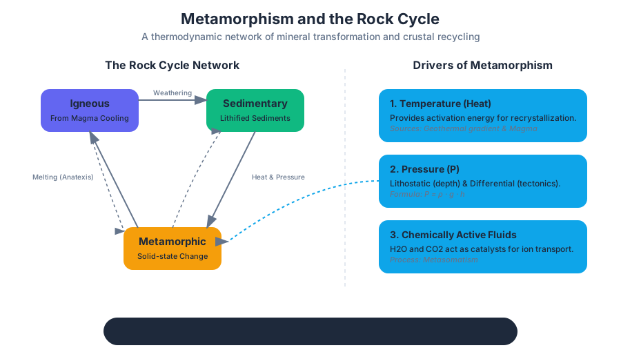
Metamorphism is the process by which the mineralogy, texture, and chemical composition of a rock change in the solid state due to extreme variations in temperature, pressure, and the introduction of chemically active fluids. Unlike igneous processes, metamorphism does not involve melting; if a rock melts, it enters the igneous realm. Instead, metamorphism is a "recrystallization" event where atoms migrate through crystal lattices to form new, stable mineral assemblages.

The Rock Cycle: A Thermodynamic Network

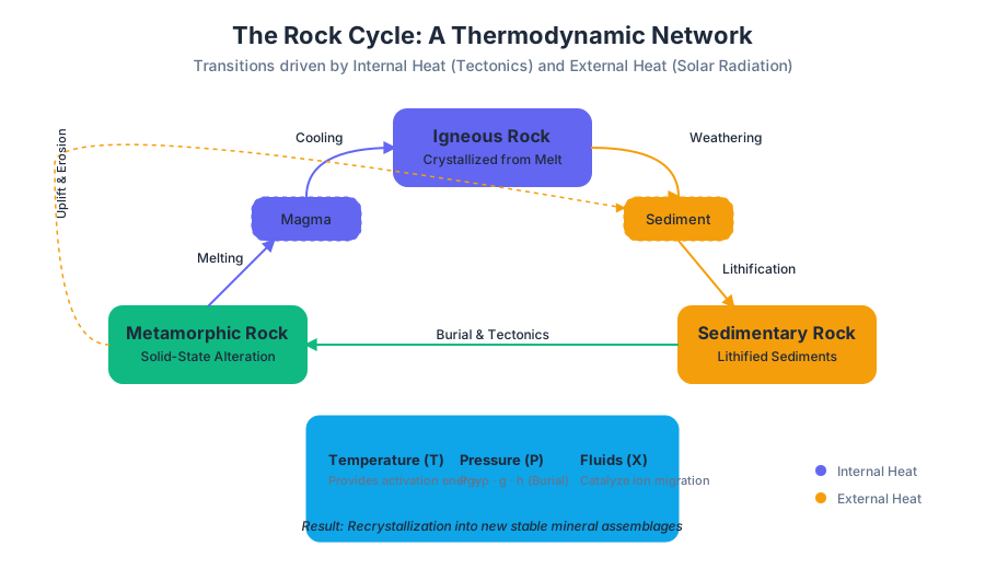
The Rock Cycle is a conceptual framework that describes the transitions through geologic time among the three main rock types: Sedimentary, Igneous, and Metamorphic. While often depicted as a simple circle, it is more accurately viewed as a complex network where any rock type can be transformed into any other, depending on the tectonic and environmental "forcing functions" applied to it.

The Fundamental Law of the Rock Cycle: No rock is permanent. The Earth is a heat engine, and the rock cycle is the physical manifestation of the planet's attempt to reach thermodynamic equilibrium in a constantly shifting environment.

Transitions and Drivers

The transitions within the cycle are driven by two primary energy sources: Internal Heat (radioactive decay and primordial heat driving plate tectonics) and External Heat (solar radiation driving the hydrologic cycle and weathering).

Transition	Process	Primary Driver
Any Rock → Sedimentary	Weathering, Erosion, Deposition, Lithification	Hydrologic Cycle / Gravity
Any Rock → Igneous	Melting (Anatexis) and Crystallization	Mantle Convection / Internal Heat
Any Rock → Metamorphic	Recrystallization under Heat and Pressure	Tectonic Burial / Magmatic Intrusion

To understand the rock cycle as a system, we can model the "residence time" of minerals in different states using a state-transition approach.

import numpy as np

class RockCycleSimulator:
    """
    A simplified Markov Chain simulation of the Rock Cycle.
    Represents the probability of a rock unit transitioning between states
    over a geologic timestep (e.g., 1 million years).
    """
    def __init__(self):
        self.states = ["Igneous", "Sedimentary", "Metamorphic", "Magma", "Sediment"]
        # Transition matrix P[i][j] = probability of moving from state i to j
        self.transition_matrix = np.array([
            [0.80, 0.05, 0.10, 0.04, 0.01], # Igneous
            [0.00, 0.70, 0.15, 0.00, 0.15], # Sedimentary
            [0.05, 0.05, 0.80, 0.10, 0.00], # Metamorphic
            [0.90, 0.00, 0.00, 0.10, 0.00], # Magma
            [0.00, 0.85, 0.00, 0.00, 0.15]  # Sediment
        ])

    def simulate(self, initial_distribution, steps=100):
        current_state = np.array(initial_distribution)
        history = [current_state]
        for _ in range(steps):
            current_state = np.dot(current_state, self.transition_matrix)
            history.append(current_state)
        return history

# Example: Starting with 100% Igneous crust
sim = RockCycleSimulator()
results = sim.simulate([1.0, 0.0, 0.0, 0.0, 0.0], steps=50)
print(f"Steady state distribution after 50Ma: {results[-1]}")

The Drivers of Metamorphism

Metamorphism is governed by three primary variables: Temperature ($T$), Pressure ($P$), and Fluid Composition ($X_{fluid}$).

1. Temperature (Heat)

Heat is the most essential agent. It provides the activation energy required for chemical reactions and the breaking of atomic bonds.

• Sources: The geothermal gradient (averaging 25°C/km) and localized magmatic intrusions.
• Effect: Increases atomic vibration, allowing ions to migrate more freely. This leads to Recrystallization (small grains joining to form larger ones) and Neocrystallization (formation of entirely new minerals).

2. Pressure

Pressure increases with depth due to the weight of overlying rock (Lithostatic Pressure).

• Lithostatic Pressure: Equal in all directions, similar to hydrostatic pressure in water. It results in a reduction of volume and the formation of high-density minerals.
• Differential Stress: Unequal pressure in different directions, typically caused by tectonic forces. This is the primary driver of Foliation.

The lithostatic pressure $P$ at depth $h$ is derived as:

P = \rho \cdot g \cdot h

Where:

• $\rho$ is the average density of the crust (~2,700 to 3,000 kg/m³)
• $g$ is the acceleration due to gravity (9.81 m/s²)
• $h$ is the depth in meters.

3. Chemically Active Fluids

Mainly water ($H_2O$) and carbon dioxide ($CO_2$) trapped in the pore spaces of sedimentary rocks or hydrated minerals. At high $P$ and $T$, these fluids become "supercritical," acting as catalysts that transport ions across great distances. This process is known as Metasomatism.

Metamorphic Grade and Facies

Metamorphic Grade is a relative term used to describe the intensity of metamorphism. It reflects the maximum $P$ and $T$ conditions a rock has experienced.

The P-T Path and Phase Boundaries

Minerals are stable only within specific $P-T$ ranges. When a rock is subjected to conditions outside its stability field, a phase transition occurs. We can describe the boundary between two mineral phases (e.g., Andalusite to Kyanite) using the Clausius-Clapeyron Equation:

\frac{dP}{dT} = \frac{\Delta S}{\Delta V}

Where:

• $dP/dT$ is the slope of the boundary on a P-T diagram.
• $\Delta S$ is the change in entropy.
• $\Delta V$ is the change in molar volume.

Metamorphic Facies

A Metamorphic Facies is a set of mineral assemblages that repeatedly associate in space and time, indicating a specific range of $P$ and $T$.

Facies	Temperature	Pressure	Tectonic Setting
Zeolite	Low (<200°C)	Low	Shallow burial
Greenschist	Moderate (300-450°C)	Moderate	Regional metamorphism (Orogeny)
Amphibolite	High (450-700°C)	Moderate/High	Deep crustal orogeny
Granulite	Very High (>700°C)	High	Base of the continental crust
Blueschist	Low/Moderate	Very High	Subduction zones (high P, low T)
Eclogite	High	Extremely High	Deep subduction (mantle depths)

Foliation: The Geometry of Stress

Foliation refers to any planar (flat) arrangement of mineral grains or structural features within a rock. It is a fundamental diagnostic tool for identifying metamorphic rocks and reconstructing tectonic history.

Mechanisms of Foliation

1. Rotation: Platy minerals (like mica) rotate until they are perpendicular to the direction of maximum stress.
2. Recrystallization: Minerals grow in a preferred orientation.
3. Pressure Solution: Ions dissolve at high-stress contact points and reprecipitate in low-stress areas (perpendicular to the stress).

The Foliation Sequence (Protolith: Shale)

As metamorphic grade increases, the texture of a pelitic (clay-rich) rock evolves:

1. Slate: Excellent Slaty Cleavage. Microscopic micas. Dull surface.
2. Phyllite: Micas grow larger; the rock develops a "sheen" or "silky luster." Surfaces are often wavy.
3. Schist: Visible mica flakes. Exhibits Schistosity. Often contains "porphyroblasts" (large crystals like garnet).
4. Gneiss: High-grade metamorphism. Ion migration results in Gneissic Banding (segregation of light silicates and dark ferromagnesian minerals).

Insight: Gneissic banding represents a high-degree of chemical segregation. The rock has almost reached its melting point, allowing minerals to migrate into distinct layers based on their chemical affinities.

Contact vs. Regional Metamorphism

The environment in which metamorphism occurs dictates the resulting rock's characteristics.

Contact (Thermal) Metamorphism

• Mechanism: "Baking" of country rock by an adjacent magma body.
• Dominant Factor: Temperature.
• Result: Non-foliated rocks (e.g., Hornfels, Quartzite, Marble).
• Aureole: The zone of alteration surrounding the intrusion. The width of the aureole depends on the size of the intrusion and the fluid content of the host rock.

Regional Metamorphism

• Mechanism: Large-scale tectonic processes, such as continental collisions or subduction.
• Dominant Factor: Both Temperature and Differential Pressure.
• Result: Foliated rocks covering thousands of square kilometers. This is where the majority of the Earth's metamorphic crust is formed.

Feature	Contact Metamorphism	Regional Metamorphism
Scale	Local (meters to kilometers)	Vast (hundreds of kilometers)
Pressure	Low (shallow depths)	High (deep burial)
Texture	Non-foliated (Granoblastic)	Foliated
Example Rock	Marble, Quartzite	Schist, Gneiss

Protolith Evolution: From Source to Product

The identity of a metamorphic rock is determined by two things: the metamorphic grade and the Protolith (the original, parent rock).

Protolith	Low Grade	Intermediate Grade	High Grade
Shale / Mudstone	Slate	Schist	Gneiss
Basalt	Greenschist	Amphibolite	Granulite / Eclogite
Limestone	Marble	Marble (coarser)	Marble (very coarse)
Sandstone	Quartzite	Quartzite	Quartzite
Granite	(Little change)	Orthogneiss	Orthogneiss

Worked Example: The Barrovian Sequence

In the late 19th century, George Barrow mapped the Scottish Highlands and noticed a predictable sequence of mineral appearances as he moved toward the core of the mountain range. This "Barrovian Sequence" serves as the gold standard for understanding regional metamorphism in pelitic rocks:

1. Chlorite Zone (Low grade)
2. Biotite Zone
3. Garnet Zone
4. Staurolite Zone
5. Kyanite Zone
6. Sillimanite Zone (High grade)

To visualize this data or analyze mineral stability in a lab setting, geologists often use thermodynamic modeling software. Below is a conceptual example of how one might call a thermodynamic library to calculate a phase boundary.

# Example: Using a hypothetical CLI tool 'geochem-sim' to 
# calculate the stability of the Al2SiO5 polymorphs.

# 1. Define the system components
geochem-sim define --system "Al2O3-SiO2"

# 2. Set the P-T range for the simulation
# Pressure: 0 to 10 kbar, Temperature: 200 to 800 C
geochem-sim set-range --p_min 0 --p_max 10 --t_min 200 --t_max 800

# 3. Run the Gibbs Free Energy minimization
geochem-sim calculate-stability --output phase_diagram.csv

# 4. Plot the results using gnuplot
gnuplot -e "set datafile separator ','; plot 'phase_diagram.csv' with lines"

Common Pitfalls and Misconceptions

1. Metamorphism vs. Weathering: While both involve mineral changes, weathering occurs at the surface (low $P$, low $T$) and involves disintegration. Metamorphism occurs at depth and involves "growth" in the solid state.
2. The "Melting" Myth: Students often think metamorphic rocks are "partially melted." If a rock melts significantly, it is a Migmatite (the bridge between metamorphic and igneous). If it melts completely, it is magma.
3. Foliation and Bedding: Foliation is a metamorphic texture; bedding is a sedimentary structure. They are rarely parallel. Foliation usually cuts across original bedding planes because tectonic stress is rarely aligned with the original depositional horizontal.
4. Isochemical Nature: Metamorphism is generally isochemical, meaning the bulk chemical composition of the rock stays the same (except for the loss of volatiles like $H_2O$). If the chemistry changes significantly due to fluid transport, it is specifically called metasomatism.

Measuring Geologic Time and Earth History

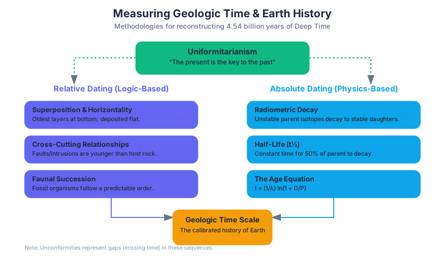
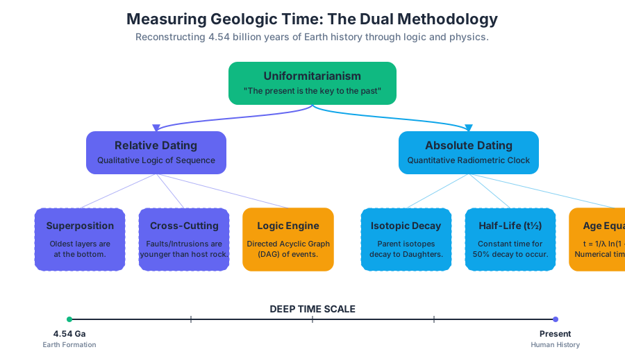
The study of Earth history is an exercise in temporal scaling. While human history is measured in decades and centuries, geologic history—often referred to as Deep Time—spans 4.54 billion years. To reconstruct this history, geologists employ two distinct but complementary methodologies: Relative Dating, which establishes the chronological order of events without necessarily determining their absolute age, and Absolute (Radiometric) Dating, which provides numerical ages in years before present.

The Philosophy of Deep Time

The foundation of modern geology rests on the principle of Uniformitarianism, famously summarized by James Hutton as "the present is the key to the past." This principle posits that the physical and chemical laws governing the universe today have remained constant throughout geologic time. Consequently, by observing modern processes like silt deposition in a river delta or the cooling of lava, geologists can infer the origins of ancient rock formations.

Uniformitarianism: The theory that changes in the earth's crust during geological history have resulted from the action of continuous and uniform processes. It stands in contrast to Catastrophism, the idea that Earth's features were formed primarily by sudden, short-lived, violent events.

---

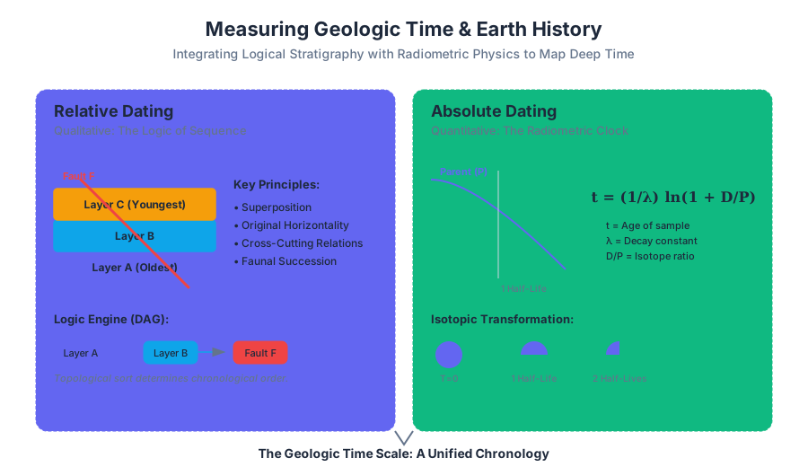
Relative Dating: The Logic of Sequence

Relative dating is the "logic-based" approach to Earth history. It does not require laboratory equipment; rather, it requires the application of several fundamental principles to "read" the stratigraphic record.

Fundamental Principles of Stratigraphy

Geologists use a set of rules, many first articulated by Nicolas Steno in the 17th century, to determine the relative timing of geologic events.

Principle	Description	Geologic Implication
Superposition	In an undeformed sequence of sedimentary rocks, each layer is older than the one above it.	Establishes a vertical timeline from bottom (old) to top (young).
Original Horizontality	Layers of sediment are generally deposited in a horizontal position.	Folded or tilted layers indicate post-depositional tectonic activity.
Lateral Continuity	Sedimentary layers extend in all directions until they thin out or reach the edge of the basin.	Allows for the correlation of rock units across valleys or canyons.
Cross-Cutting Relationships	If a fault or igneous intrusion cuts through another rock body, the fault/intrusion must be younger.	Identifies the timing of tectonic or magmatic events relative to host rock.
Inclusions	Fragments of one rock unit (xenoliths or clasts) contained within another must be older than the host rock.	Helps distinguish between a lava flow and a later sill intrusion.
Faunal Succession	Fossil organisms succeed one another in a definite and determinable order.	Enables global correlation of strata based on biological evolution.

Unconformities: Gaps in the Record

The geologic record is rarely continuous. Unconformities represent periods of non-deposition or erosion, effectively acting as "missing pages" in Earth's history book.

1. Angular Unconformity: Tilted or folded sedimentary rocks are overlain by younger, more flat-lying strata.
2. Disconformity: A gap in the rock record between parallel layers of sedimentary rock, usually caused by erosion.
3. Nonconformity: Younger sedimentary rocks are deposited directly on top of older metamorphic or igneous rocks.

Implementation: Relative Age Logic Engine

In computational geology, we can model these relationships as a Directed Acyclic Graph (DAG) where nodes represent rock units and edges represent "older than" relationships.

class GeologicUnit:
    def __init__(self, name, unit_type):
        self.name = name
        self.unit_type = unit_type # 'sedimentary', 'igneous', 'fault'
        self.older_than = []

    def add_relationship(self, younger_unit):
        """Applies the logic of cross-cutting or superposition."""
        younger_unit.older_than.append(self)

def resolve_chronology(units):
    """
    Performs a topological sort to determine the sequence of events.
    """
    visited = set()
    stack = []

    def visit(node):
        if node not in visited:
            visited.add(node)
            for predecessor in node.older_than:
                visit(predecessor)
            stack.append(node.name)

    for unit in units:
        visit(unit)
    
    return stack[::-1] # Returns sequence from oldest to youngest

# Example: Fault F cuts through Layer A and Layer B. Layer B is above Layer A.
layer_a = GeologicUnit("Layer A", "sedimentary")
layer_b = GeologicUnit("Layer B", "sedimentary")
fault_f = GeologicUnit("Fault F", "fault")

layer_b.add_relationship(layer_a) # Superposition: B is younger than A
fault_f.add_relationship(layer_a) # Cross-cutting: F is younger than A
fault_f.add_relationship(layer_b) # Cross-cutting: F is younger than B

print(f"Chronological Order: {resolve_chronology([layer_a, layer_b, fault_f])}")

---

Absolute Dating: The Radiometric Clock

While relative dating provides the order, Radiometric Dating provides the timestamp. This method relies on the spontaneous decay of unstable atomic nuclei (isotopes).

The Physics of Decay

A radioactive parent isotope decays into a stable daughter isotope at a constant, measurable rate called a half-life ($t_{1/2}$). The half-life is the time required for half of the parent nuclei in a sample to decay.

The Age Equation: The age ($t$) of a mineral can be calculated using the decay constant ($\lambda$) and the current ratio of daughter ($D$) to parent ($P$) atoms.

t = \frac{1}{\lambda} \ln \left( 1 + \frac{D}{P} \right)

Where the decay constant $\lambda$ is related to the half-life by:

\lambda = \frac{\ln(2)}{t_{1/2}} \approx \frac{0.693}{t_{1/2}}

Common Isotopic Systems

Different isotopes are used depending on the expected age and the composition of the material.

Isotope System	Parent $\rightarrow$ Daughter	Half-Life (Years)	Effective Dating Range	Typical Materials
Uranium-238	$^{238}U \rightarrow ^{206}Pb$	4.47 Billion	10M – 4.6B years	Zircon, Apatite
Potassium-40	$^{40}K \rightarrow ^{40}Ar$	1.25 Billion	100k – 4.6B years	Micas, Feldspar, Hornblende
Rubidium-87	$^{87}Rb \rightarrow ^{87}Sr$	48.8 Billion	10M – 4.6B years	Micas, Metamorphic rocks
Carbon-14	$^{14}C \rightarrow ^{14}N$	5,730	100 – 50,000 years	Organic matter (bone, wood)

The "Resetting" of the Clock

A critical concept in radiometric dating is the Closure Temperature. Radiometric clocks in igneous rocks start when the mineral cools below a specific temperature, "locking in" the parent and daughter isotopes. If a rock is later reheated (metamorphism), the daughter isotopes may escape, effectively "resetting" the clock and providing the age of the metamorphic event rather than the original crystallization.

Data Acquisition Workflow

To obtain a date, geologists follow a rigorous analytical pipeline.

# Hypothetical workflow for U-Pb dating using a Mass Spectrometer CLI
$ geochron-tool --import sample_Zircon_001.raw
$ geochron-tool --calibrate --standard NIST610
$ geochron-tool --calculate-ratios --parent U238 --daughter Pb206
$ geochron-tool --plot-concordia --sample Zircon_001

# Output:
# Best fit age: 420.5 +/- 1.2 Ma
# MSWD (Mean Square of Weighted Deviates): 1.05 (Good fit)

---

The Geologic Time Scale

The Geologic Time Scale (GTS) is the "calendar" of Earth's history. It is a hierarchical system that divides time based on major geological and biological events.

Hierarchy of Time

1. Eons: The largest division (e.g., Phanerozoic, Proterozoic, Archean, Hadean).
2. Eras: Subdivisions of Eons (e.g., Paleozoic, Mesozoic, Cenozoic).
3. Periods: Subdivisions of Eras (e.g., Jurassic, Cretaceous).
4. Epochs: Subdivisions of Periods (e.g., Holocene, Pleistocene).

Key Transitions in Earth History

The GTS is not divided into equal time blocks; instead, boundaries are defined by significant changes in the fossil record or global geochemistry.

• The Precambrian (88% of Earth history): Includes the Hadean, Archean, and Proterozoic eons. This era saw the formation of Earth, the rise of oxygen (Great Oxygenation Event), and the first multicellular life.
• The Cambrian Explosion: The beginning of the Phanerozoic Eon, marked by a rapid diversification of life forms with hard shells.
• The Great Dying (Permian-Triassic Boundary): The largest mass extinction in history, marking the end of the Paleozoic Era.
• The Age of Dinosaurs (Mesozoic): Ended by the K-Pg extinction event 66 million years ago.

---

Evolution and Mass Extinctions

The fossil record provides the biological context for geologic time. Biostratigraphy uses the presence of Index Fossils to correlate rock layers across vast distances.

Index Fossil: A fossil that is useful for dating and correlating the strata in which it is found. A good index fossil must be:

1. Geographically widespread.
2. Easily identifiable.
3. Short-lived (existed for a narrow slice of geologic time).
4. Abundant.

The "Big Five" Mass Extinctions

Mass extinctions serve as the primary markers for the boundaries between geologic Eras and Periods.

Extinction Event	Time (Ma)	Major Groups Lost	Probable Cause
End Ordovician	444	85% of marine species	Glaciation and falling sea levels
Late Devonian	365	75% of species	Global cooling, ocean anoxia
End Permian	252	96% of marine, 70% of terrestrial	Siberian Traps volcanism, CO2 spike
End Triassic	201	80% of species	CAMP volcanism, climate change
End Cretaceous	66	Dinosaurs, ammonites	Asteroid impact (Chicxulub)

Querying the Paleobiology Database

Modern paleontologists use SQL-based databases to track the rise and fall of taxa over time.

-- Query to find the diversity of Brachiopods across the P-T Boundary
SELECT 
    interval_name, 
    COUNT(DISTINCT genus) AS genus_count
FROM 
    paleobio_data
WHERE 
    taxon_group = 'Brachiopoda' 
    AND interval_name IN ('Capitanian', 'Wuchiapingian', 'Changhsingian', 'Induan')
GROUP BY 
    interval_name
ORDER BY 
    age_ma DESC;

---

Common Pitfalls and Misconceptions

1. Dating Sedimentary Rocks Directly

A common mistake is attempting to radiometrically date a sandstone to find out when it was deposited. Radiometric dating of a sand grain (e.g., a zircon) tells you when that specific grain crystallized in its original igneous source rock, not when it was deposited as sediment. To date sedimentary layers, geologists must date interbedded volcanic ash layers (tuffs) or use relative dating principles.

2. The Meaning of "Absolute"

"Absolute" dating does not mean "perfect." Every radiometric date comes with an error margin (e.g., $66.0 \pm 0.5$ Ma). These margins are calculated based on analytical precision and potential contamination.

3. Carbon-14 Limitations

Carbon-14 is often mentioned in popular media for dating everything from dinosaurs to the Earth. However, due to its short half-life (5,730 years), it is useless for anything older than approximately 50,000 years. Dinosaurs (which died out 66 million years ago) cannot be dated with Carbon-14.

4. The "Incomplete" Record

Charles Darwin famously noted that the geologic record is like a book with most of its pages torn out and only a few lines remaining on the pages that are left. This is due to the constant recycling of the Earth's crust via plate tectonics and erosion.

---

Summary of Methodological Integration

The reconstruction of Earth history is an iterative process. A geologist might find a fossil (Relative Dating), identify the rock layer's position relative to a fault (Relative Dating), and then find a volcanic ash layer nearby that can be dated in a lab (Absolute Dating). By combining these data points, we create the high-resolution timeline used to understand climate change, evolution, and the movement of continents.

Earth's Interior and Plate Tectonics

The theory of Plate Tectonics serves as the "Grand Unified Theory" of geology. It provides a robust physical framework that links seemingly disparate phenomena—such as the distribution of fossilized tropical plants in Antarctica, the deep-focus earthquakes of the Pacific Rim, and the chemistry of mid-ocean ridge basalts—into a single, coherent system. At its core, plate tectonics describes the Earth's surface as a mosaic of rigid segments, or lithospheric plates, that move relative to one another over a ductile substratum. This movement is the primary mechanism by which Earth loses its internal heat to space.

The Stratified Earth: Compositional vs. Rheological Layers

To understand plate tectonics, one must first distinguish between the Earth's layers based on chemical composition (what they are made of) versus their rheology or mechanical behavior (how they deform).

Compositional Layers

The Earth is chemically differentiated into three primary units:

1. Crust: The outermost "skin," rich in silica and aluminum. It is divided into thin, dense oceanic crust (basaltic) and thick, buoyant continental crust (granitic).
2. Mantle: A 2,900 km thick layer of silicate rock rich in magnesium and iron (peridotite). It comprises about 84% of Earth's volume.
3. Core: A dense metallic center composed primarily of iron and nickel.

Rheological Layers

Plate tectonics is concerned primarily with the mechanical properties of the upper 700 km.

• Lithosphere: The cool, rigid outer shell. It includes the crust and the uppermost portion of the mantle. It behaves elastically or brittly; when stressed, it breaks (earthquakes).
• Asthenosphere: Located beneath the lithosphere, this layer is "plastic" or ductile. While it is solid rock, it is near its melting point, allowing it to flow over geologic timescales.
• Mesosphere: The lower mantle, where high pressure increases the strength of the rock despite higher temperatures.
• Outer Core: Liquid metal; its flow generates Earth's magnetic field.
• Inner Core: Solid metal due to extreme pressure.

Layer	Depth (km)	State	Composition	Density (g/cm³)
Continental Crust	30–70	Rigid	Granitic (Felsic)	2.7
Oceanic Crust	5–10	Rigid	Basaltic (Mafic)	3.0
Lithospheric Mantle	Crust to ~100	Rigid	Peridotite (Ultramafic)	3.3
Asthenosphere	100–660	Plastic/Ductile	Peridotite	3.4–4.4
Outer Core	2890–5150	Liquid	Fe-Ni Alloy	9.9–12.2
Inner Core	5150–6371	Solid	Fe-Ni Alloy	12.8–13.1

The Physics of Isostasy

The lithosphere "floats" on the asthenosphere according to the principle of Isostasy, which is essentially Archimedes' Principle applied to the Earth's crust. The depth to which a plate sinks depends on its thickness and its density relative to the underlying mantle.

The Airy Isostasy Model: States that the pressure at a certain "compensation depth" must be equal everywhere. For a mountain of height $h$ and density $\rho_c$ floating in a mantle of density $\rho_m$, the "root" $r$ extending into the mantle is calculated as: $$r = h \frac{\rho_c}{\rho_m - \rho_c}$$

The following Python script demonstrates how to calculate the required crustal root for a given mountain range height using the Airy Isostasy model.

import numpy as np

def calculate_crustal_root(elevation_m, rho_crust=2700, rho_mantle=3300):
    """
    Calculates the depth of the crustal root (r) required to support 
    a given surface elevation (h) based on Airy Isostasy.
    
    Parameters:
    elevation_m (float): Height of the mountain above sea level in meters.
    rho_crust (float): Density of the crust in kg/m^3. Default is 2700 (granite).
    rho_mantle (float): Density of the mantle in kg/m^3. Default is 3300 (peridotite).
    
    Returns:
    float: The thickness of the root in meters.
    """
    if rho_mantle <= rho_crust:
        raise ValueError("Mantle density must be greater than crust density.")
        
    # Airy formula: r = h * (rho_c / (rho_m - rho_c))
    root_depth = elevation_m * (rho_crust / (rho_mantle - rho_crust))
    
    return root_depth

# Example: The Himalayas (avg elevation ~5000m)
h_himalayas = 5000
root = calculate_crustal_root(h_himalayas)

print(f"For a mountain height of {h_himalayas}m:")
print(f"Required Root Depth: {root:.2f} meters")
print(f"Total Crustal Thickness: {h_himalayas + root:.2f} meters")

Mantle Convection: The Engine of Tectonics

Plate movement is driven by the transfer of heat from the Earth's interior to its surface. This occurs primarily through convection—the physical movement of hot, less-dense material upward and cool, denser material downward.

The Rayleigh Number ($Ra$)

Whether a fluid (or a plastic solid like the mantle) will undergo convection is determined by the Rayleigh Number. If $Ra$ exceeds a critical value (typically around 1000 for the mantle), convection begins.

Ra = \frac{\alpha g \Delta T d^3}{\kappa \nu}

Where:

• $\alpha$: Thermal expansion coefficient
• $g$: Acceleration due to gravity
• $\Delta T$: Temperature difference across the layer
• $d$: Depth of the layer
• $\kappa$: Thermal diffusivity
• $\nu$: Kinematic viscosity

In the mantle, $\nu$ is extremely high ($10^{19}$ to $10^{21}$ Pa·s), but the depth $d$ is so large that $Ra$ is estimated to be $10^6$ to $10^8$, far exceeding the threshold for convection.

Driving Forces

While convection cells provide the general motion, two specific gravitational forces dominate plate movement:

1. Slab Pull: As a subducting plate sinks into the mantle, its high density (due to cooling and phase changes like the basalt-to-eclogite transition) pulls the rest of the plate behind it. This is considered the strongest force.
2. Ridge Push: The elevated position of a mid-ocean ridge creates a gravitational gradient, causing the lithosphere to "slide" away from the ridge axis.

Plate Boundary Dynamics

The interactions between plates occur at their boundaries. These interactions are classified into three fundamental types, each characterized by specific geologic structures and seismic signatures.

1. Divergent Boundaries (Constructive)

Plates move apart, and new lithosphere is created by the upwelling of mantle material.

• Oceanic: Mid-Ocean Ridges (e.g., Mid-Atlantic Ridge). Characterized by shallow earthquakes and basaltic volcanism.
• Continental: Rift Valleys (e.g., East African Rift). Can eventually lead to the formation of a new ocean basin.

2. Convergent Boundaries (Destructive)

Plates collide, leading to the recycling of lithosphere or mountain building.

• Ocean-Ocean: One plate subducts beneath the other, forming a Volcanic Island Arc (e.g., Japan, Marianas).
• Ocean-Continent: The denser oceanic plate subducts under the continental plate, forming a Continental Volcanic Arc (e.g., The Andes).
• Continent-Continent: Neither plate is dense enough to subduct deeply; instead, the crust thickens and is thrust upward to form massive mountain ranges (e.g., The Himalayas).

3. Transform Boundaries (Conservative)

Plates slide past each other horizontally. No lithosphere is created or destroyed.

• Example: The San Andreas Fault.
• These boundaries facilitate the "stepping" of mid-ocean ridges and accommodate the movement of plates on a spherical Earth.

Boundary Type	Stress Type	Volcanism?	Earthquakes	Key Feature
Divergent	Tension	Yes (Mafic)	Shallow, Weak	Central Rift Valley
Convergent (Subduction)	Compression	Yes (Intermediate)	Shallow to Deep (Benioff Zone)	Trench / Arc
Convergent (Collision)	Compression	No	Shallow to Medium	High Mountains
Transform	Shear	No	Shallow, Strong	Strike-slip fault

Kinematics: Describing Plate Motion

Because plates move on the surface of a sphere, their motion cannot be described by simple linear vectors. Instead, we use Euler’s Rotation Theorem, which states that any displacement of a rigid body on the surface of a sphere can be described as a rotation around a fixed axis passing through the center of the sphere. This axis intersects the surface at the Euler Pole.

Calculating Relative Velocity

The velocity $v$ of a point on a plate at a distance $R$ from the Earth's center is: $$v = \omega \times r$$ Where $\omega$ is the angular velocity vector and $r$ is the position vector of the point. Consequently, the linear velocity of a plate is zero at the Euler pole and reaches its maximum at the "equator" relative to that pole.

To analyze plate motions, geologists often query large datasets of GPS station coordinates. Below is a conceptual SQL schema and query used to track the displacement of geodetic markers over time.

-- Schema for tracking GPS station displacement
CREATE TABLE gps_stations (
    station_id VARCHAR(10) PRIMARY KEY,
    plate_name VARCHAR(50),
    latitude DECIMAL(9,6),
    longitude DECIMAL(9,6)
);

CREATE TABLE station_measurements (
    measurement_id SERIAL PRIMARY KEY,
    station_id VARCHAR(10) REFERENCES gps_stations(station_id),
    observation_time TIMESTAMP,
    north_displacement_mm DECIMAL(10,3),
    east_displacement_mm DECIMAL(10,3),
    up_displacement_mm DECIMAL(10,3)
);

-- Query to calculate average annual velocity for the Pacific Plate
SELECT 
    g.plate_name,
    AVG(m.north_displacement_mm) AS avg_north_velocity_mm_yr,
    AVG(m.east_displacement_mm) AS avg_east_velocity_mm_yr,
    SQRT(POWER(AVG(m.north_displacement_mm), 2) + POWER(AVG(m.east_displacement_mm), 2)) AS total_magnitude_mm_yr
FROM 
    gps_stations g
JOIN 
    station_measurements m ON g.station_id = m.station_id
WHERE 
    g.plate_name = 'Pacific'
    AND m.observation_time >= '2022-01-01' 
    AND m.observation_time < '2023-01-01'
GROUP BY 
    g.plate_name;

Mantle Plumes and Hotspots

While plate tectonics explains most volcanic activity, it does not account for intraplate volcanism—volcanoes that appear in the middle of a plate, far from any boundary. The most widely accepted explanation is the Mantle Plume hypothesis.

Mechanics of Plumes

A mantle plume is a buoyant mass of hot rock rising from the core-mantle boundary (the D'' layer). As the plume head reaches the base of the lithosphere, it undergoes decompression melting, creating a hotspot.

• Stationary Source: Plumes are relatively stationary compared to the rapidly moving lithospheric plates.
• Hotspot Tracks: As a plate moves over a stationary plume, it creates a chain of volcanoes that get progressively older as you move away from the current hotspot location (e.g., the Hawaiian-Emperor Seamount Chain).

The Wilson Cycle

The opening and closing of ocean basins is a cyclical process driven by these forces:

1. Embryonic: Continental rifting (East Africa).
2. Juvenile: Opening of a narrow sea (Red Sea).
3. Mature: Wide ocean basin with passive margins (Atlantic).
4. Declining: Subduction begins; ocean starts to close (Pacific).
5. Terminal: Narrowing sea due to collision (Mediterranean).
6. Suturing: Continent-continent collision (Himalayas).

Common Pitfalls and Misconceptions

• "Plates float on a sea of liquid magma": This is perhaps the most common error. The mantle is solid. It flows via solid-state creep (dislocation climb and diffusion) at the rate of centimeters per year. Only in very specific areas (mid-ocean ridges, subduction zones, hotspots) does the mantle melt to form magma.
• Confusing Crust and Lithosphere: The crust is a chemical definition; the lithosphere is a mechanical one. The lithosphere contains the crust plus the uppermost rigid mantle.
• The "Conveyor Belt" Misconception: While mantle convection is the ultimate driver, the plates are not merely passive passengers on a conveyor belt. Because of slab pull, the plates are active participants in the convective system—they are the cold, upper boundary layer of the convection cells themselves.

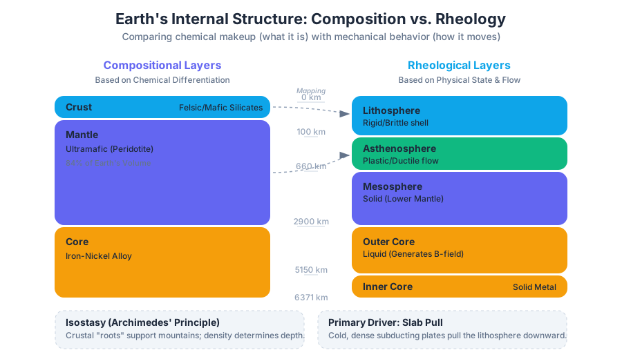
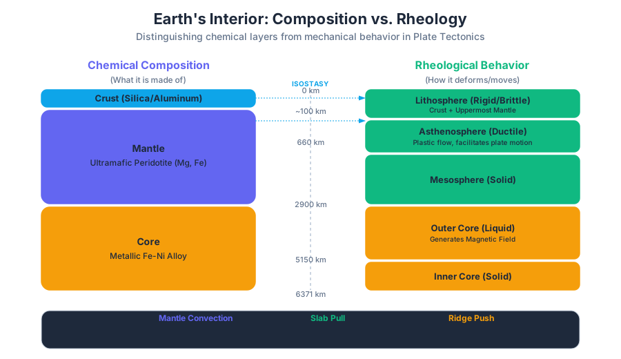
Earthquakes and Geological Structures

The Earth’s crust is not a static shell but a dynamic medium under constant internal pressure. When tectonic forces—driven by mantle convection and plate movements—exert pressure on rock masses, the crust undergoes deformation. This deformation manifests as the bending, breaking, and tilting of rock layers, creating the complex geological structures we observe today. Seismology is the study of the energy released when these rocks finally fail, sending shockwaves through the planetary interior.

Mechanics of Crustal Deformation: Stress and Strain

To understand why a mountain range folds or a fault ruptures, we must first distinguish between the force applied and the resulting change in the rock.

• Stress ($\sigma$ or $\tau$): The force applied per unit area. It is a vector quantity that can be resolved into normal stress (perpendicular to a surface) and shear stress (parallel to a surface).
• Strain ($\epsilon$): The physical change in shape or volume of the rock in response to stress.

Rocks respond to stress in three distinct stages:

1. Elastic Deformation: The rock deforms but returns to its original shape once stress is removed. This is the "spring" mechanism that stores energy for earthquakes.
2. Ductile (Plastic) Deformation: Beyond the elastic limit, the rock flows or bends permanently without breaking. This typically occurs at high temperatures and pressures deep within the crust.
3. Brittle Failure: If stress is applied rapidly or the rock is cold (near the surface), it fractures. This is the primary cause of faults and earthquakes.

Stress Type	Tectonic Environment	Primary Resulting Structure	Dimensional Change
Compression	Convergent Boundaries	Folds, Reverse Faults	Shortening and Thickening
Tension	Divergent Boundaries	Normal Faults	Lengthening and Thinning
Shear	Transform Boundaries	Strike-Slip Faults	Lateral Displacement

The Mohr-Coulomb Failure Criterion

In structural engineering and geology, we use the Mohr-Coulomb criterion to predict when a rock will transition from elastic behavior to brittle failure. The shear strength of a rock ($\tau$) is defined by its internal cohesion ($C$) and the angle of internal friction ($\phi$).

import numpy as np
import matplotlib.pyplot as plt

def plot_mohr_circle(sigma_1, sigma_3, cohesion, phi_deg):
    """
    Visualizes the Mohr's Circle for a given stress state 
    and the Mohr-Coulomb failure envelope.
    """
    phi = np.radians(phi_deg)
    center = (sigma_1 + sigma_3) / 2
    radius = (sigma_1 - sigma_3) / 2
    
    # Generate circle points
    theta = np.linspace(0, 2*np.pi, 100)
    x = center + radius * np.cos(theta)
    y = radius * np.sin(theta)
    
    # Generate failure envelope: tau = C + sigma * tan(phi)
    sigma_env = np.linspace(0, sigma_1 + 10, 100)
    tau_env = cohesion + sigma_env * np.tan(phi)
    
    plt.figure(figsize=(10, 6))
    plt.plot(x, y, label="Mohr's Circle (Stress State)")
    plt.plot(sigma_env, tau_env, 'r--', label="Failure Envelope")
    plt.axhline(0, color='black', lw=1)
    plt.xlabel("Normal Stress (σ)")
    plt.ylabel("Shear Stress (τ)")
    plt.title("Brittle Failure Analysis")
    plt.legend()
    plt.grid(True)
    plt.axis('equal')
    plt.show()

# Example: High compression (100MPa) vs low confining pressure (20MPa)
plot_mohr_circle(sigma_1=100, sigma_3=20, cohesion=10, phi_deg=30)

Geological Structures: Folds

Folds are the result of ductile deformation under compressional stress. They are most commonly found in the roots of mountain belts where heat and pressure allow rock to behave like a viscous fluid over millions of years.

Anatomy of a Fold

• Hinge Line: The line of maximum curvature on a folded surface.
• Axial Plane: An imaginary plane that divides the fold as symmetrically as possible, connecting the hinge lines of successive layers.
• Limbs: The "sides" of the fold on either side of the axial plane.

Primary Fold Types

1. Anticlines: Arch-like folds where the limbs dip away from the hinge. Crucially, the oldest rocks are found in the core of the fold.
2. Synclines: Trough-like folds where the limbs dip toward the hinge. The youngest rocks are found in the core.
3. Monoclines: A step-like fold in otherwise horizontal sedimentary strata, often caused by a deep-seated fault that does not reach the surface.

The Rule of Superposition in Folding: In an upright (non-overturned) fold, the relative age of the strata is the most reliable way to distinguish an anticline from a syncline, especially when the surface topography has been eroded flat.

Geological Structures: Faults

Faults are fractures in the crust along which significant displacement has occurred. They are the primary sources of seismic activity.

Dip-Slip Faults

Movement is primarily vertical, parallel to the dip of the fault plane.

• Normal Faults: The hanging wall (the block above the fault) moves down relative to the footwall. This indicates tensional stress (crustal stretching).
• Reverse Faults: The hanging wall moves up relative to the footwall. This indicates compressional stress.
• Thrust Faults: A low-angle reverse fault (dip < 45°). These are responsible for massive crustal shortening in mountain ranges like the Himalayas.

Strike-Slip Faults

Movement is primarily horizontal.

• Right-Lateral (Dextral): If you stand on one side, the opposite side appears to have moved to the right.
• Left-Lateral (Sinistral): The opposite side appears to have moved to the left.

Fault Type	Stress Regime	Tectonic Setting	Example
Normal	Tension	Mid-Ocean Ridges, Basin & Range	East African Rift
Reverse	Compression	Subduction Zones	Andes Mountains
Strike-Slip	Shear	Transform Boundaries	San Andreas Fault

Seismology: The Science of Earthquakes

An earthquake is the sudden release of stored elastic strain energy. According to the Elastic Rebound Theory, rocks on opposite sides of a fault are subjected to force and shift elastically until they reach their internal strength limit. At the moment of rupture (the focus or hypocenter), the rocks snap back to an unstrained state, releasing energy as seismic waves.

Seismic Wave Mechanics

Seismic waves are categorized into Body Waves (traveling through the Earth's interior) and Surface Waves (traveling along the crust).

1. P-waves (Primary): Longitudinal/Compressional waves. They are the fastest and can travel through solids, liquids, and gases.
2. S-waves (Secondary): Transverse/Shear waves. They move slower than P-waves and cannot travel through liquids because liquids have no shear strength. This property allowed geologists to deduce that the Earth's outer core is liquid.

\text{P-wave Velocity: } V_p = \sqrt{\frac{K + \frac{4}{3}\mu}{\rho}}
\quad \quad
\text{S-wave Velocity: } V_s = \sqrt{\frac{\mu}{\rho}}

Where:

• $K$ = Bulk Modulus (resistance to compression)
• $\mu$ = Shear Modulus (rigidity)
• $\rho$ = Density

Insight: Since $\mu = 0$ in a liquid, the formula for $V_s$ becomes zero, explaining why S-waves are blocked by the outer core (the S-wave Shadow Zone).

Wave Type	Particle Motion	Velocity	Damage Potential
P-Wave	Parallel to propagation (Push-Pull)	Fast (~6-8 km/s)	Low
S-Wave	Perpendicular to propagation (Shake)	Medium (~3-4 km/s)	Moderate
Rayleigh	Elliptical (Rolling)	Slow	Very High
Love	Side-to-side (Horizontal shear)	Slow	Very High

Locating an Epicenter

The distance to an earthquake is determined by the time lag between the arrival of the P-wave and the S-wave ($S-P$ interval). By using data from at least three seismic stations, the epicenter can be located via triangulation.

Subsurface Deduction and Mapping

Geologists cannot see beneath the Earth's surface directly. Instead, they use surface measurements of Strike and Dip to project structures into the third dimension.

• Strike: The compass direction of a line formed by the intersection of a tilted rock layer with a horizontal plane.
• Dip: The angle of inclination of the rock layer, measured downward from the horizontal plane, perpendicular to the strike.

The Rule of Vs

When a V-shaped outcrop pattern appears on a map where a bed crosses a stream valley:

• For horizontal beds, the "V" points upstream.
• For beds dipping upstream, the "V" points upstream (narrower).
• For vertical beds, there is no "V"; the outcrop is a straight line.

Practical Data Acquisition

Modern seismologists use automated tools to query global earthquake databases for structural analysis.

# Example: Querying the USGS Earthquake API for events 
# greater than Magnitude 6.0 in the last 30 days.

curl -X GET "https://earthquake.usgs.gov/fdsnws/event/1/query?format=geojson&starttime=2023-10-01&minmagnitude=6" \
     -H "accept: application/json" | jq '.features[] | {place: .properties.place, mag: .properties.mag, time: .properties.time}'

Seismic Hazards and Risk Mitigation

The danger of an earthquake is not just the magnitude, but the local geological conditions.

• Liquefaction: Unconsolidated, water-saturated sediments lose their strength during shaking and behave like a liquid, causing buildings to sink.
• Amplification: Soft soils (like bay mud) amplify seismic waves compared to hard bedrock.
• Tsunamis: Vertical displacement of the seafloor (usually via thrust faults in subduction zones) displaces the entire water column, creating long-period waves that grow in height as they approach the shore.

Magnitude vs. Intensity

It is a common pitfall to confuse the Moment Magnitude Scale ($M_w$) with the Modified Mercalli Intensity (MMI) Scale.

Scale	Measure	Type	Range
Moment Magnitude	Energy released	Quantitative/Logarithmic	1.0 - 10.0+
Modified Mercalli	Observed damage/shaking	Qualitative/Subjective	I - XII

Summary of Subsurface Interpretation

To reconstruct the history of a region, geologists combine these concepts into a Cross-Section. By applying the Principle of Cross-Cutting Relationships, we know that a fault or an igneous intrusion must be younger than the rock layers it cuts through. Similarly, if a fold is cut by a fault, the folding event occurred first.

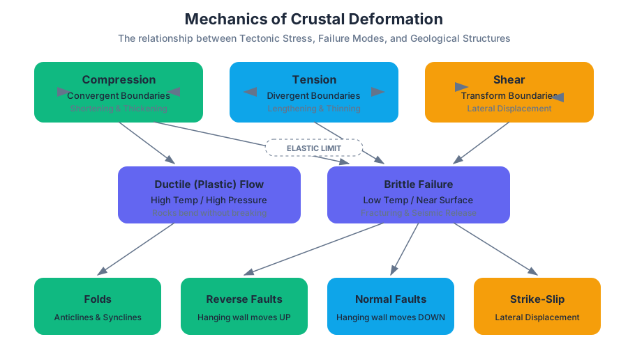
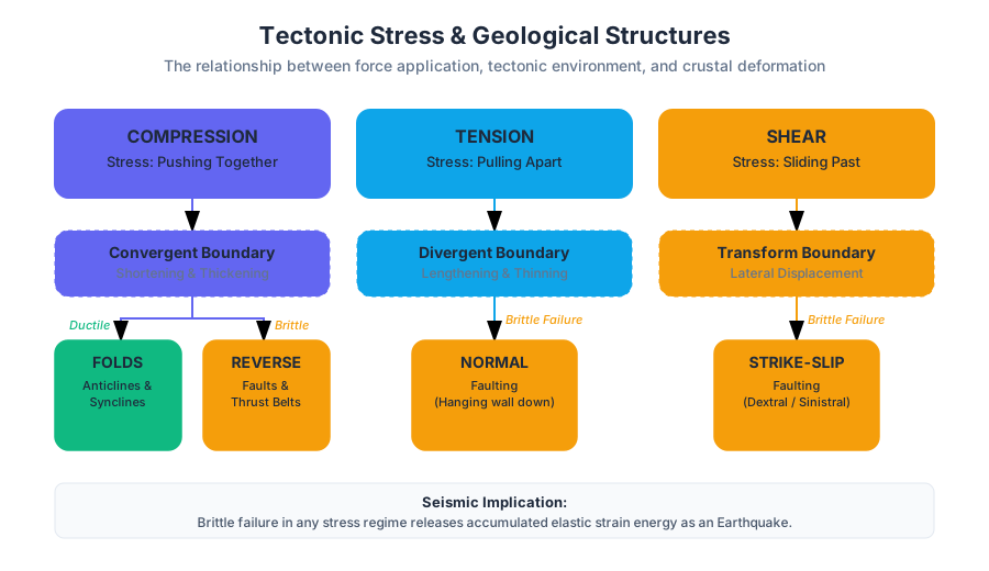
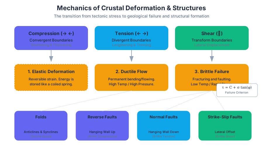
Hydrology: Streams, Floods, and Groundwater

Hydrology is the multidisciplinary study of the movement, distribution, and quality of water on Earth. It serves as the connective tissue between geology, meteorology, and ecology. In the context of Earth sciences, water is the primary architect of the landscape—a relentless agent of erosion, transport, and deposition that reshapes the crust over both millisecond and millennial timescales.

While the "Hydrologic Cycle" is often taught as a simple loop of evaporation and precipitation, the reality is a complex system of fluxes and storages. This section dives deep into the mechanics of surface water systems (streams and rivers) and the hidden dynamics of subsurface reservoirs (groundwater), exploring the physical laws that govern their behavior and the hazards they pose to human civilization.

Drainage Basins and Stream Systems

A drainage basin (or watershed) is the fundamental unit of hydrology. It is the total land area that contributes water to a specific stream or river system. These basins are hierarchical; a small creek has its own basin, which is nested within the larger basin of a major river like the Mississippi or the Amazon.

The Anatomy of a Basin

Basins are separated by topographical highs known as drainage divides. Water falling on one side of the divide flows into one catchment, while water on the other side enters a different system. Within these basins, streams organize into networks that reflect the underlying geology and climate.

The Law of Stream Numbers: In a mature drainage system, there is a highly regular inverse relationship between the stream order and the number of stream segments of that order. This fractal-like organization ensures efficient transport of water and sediment.

Stream Dynamics and Sediment Transport

Streams perform three primary geological tasks: erosion, transportation, and deposition. The energy available for these tasks is determined by the stream gradient (slope) and the discharge ($Q$), defined as the volume of water passing a point per unit of time.

Feature	Description	Primary Energy State
Headwaters	Steep gradient, V-shaped valleys, high velocity relative to bed roughness.	High Potential Energy; Erosional dominance.
Trunk Stream	Moderate gradient, meandering or braided patterns, high discharge.	Balanced; Transport dominance.
Mouth/Delta	Near-zero gradient, velocity drops as it enters a standing body of water.	Low Kinetic Energy; Depositional dominance.

Implementation: Calculating Stream Discharge

To understand the power of a stream, engineers use the Manning Equation to estimate velocity based on channel geometry and roughness.

import math

def calculate_manning_velocity(n, R, S):
    """
    Calculates the flow velocity in an open channel using Manning's Equation.
    
    Parameters:
    n (float): Manning's roughness coefficient (e.g., 0.03 for clean rivers)
    R (float): Hydraulic radius (Area / Wetted Perimeter) in meters
    S (float): Channel slope (m/m)
    
    Returns:
    v (float): Velocity in m/s
    """
    if n <= 0 or R <= 0 or S <= 0:
        raise ValueError("Parameters must be positive non-zero values.")
        
    # v = (1/n) * R^(2/3) * S^(1/2)
    velocity = (1.0 / n) * math.pow(R, 2/3) * math.pow(S, 0.5)
    return velocity

# Example: A gravel-bed stream with R=2.5m, Slope=0.005, Roughness=0.04
v = calculate_manning_velocity(0.04, 2.5, 0.005)
print(f"Calculated Stream Velocity: {v:.2f} m/s")

Groundwater: The Hidden Reservoir

Groundwater represents approximately 98% of all liquid freshwater on Earth. It is not found in "underground lakes" (except in rare cavernous limestone), but rather within the microscopic pores of soil and the fractures of bedrock.

Porosity and Permeability

The ability of a geological material to hold and transmit water is defined by two distinct but related properties:

1. Porosity: The percentage of the total volume of a rock or sediment that consists of open spaces (voids).
2. Permeability: The capacity of a material to transmit a fluid. This depends on the size of the pores and how well they are interconnected.

Material	Porosity (%)	Permeability	Hydrologic Role
Unconsolidated Gravel	25–40%	Very High	Excellent Aquifer
Sandstone	5–30%	Moderate to High	Common Aquifer
Clay	40–70%	Very Low	Aquitard (blocks flow)
Unfractured Granite	<1%	Negligible	Aquiclude (impermeable)
Fractured Shale	0–10%	Low to Moderate	Variable

The Water Table and Zones of Saturation

As meteoric water (rain/snow) infiltrates the ground, it moves through the unsaturated zone (or vadose zone), where pores contain both air and water. Eventually, it reaches the saturated zone (or phreatic zone), where all pores are filled with water. The upper boundary of this saturated zone is the Water Table.

The water table is not flat; it typically mimics the surface topography, though in a more subdued fashion. It rises under hills and sinks toward valleys, where it often intersects the surface to form springs, lakes, or streams.

Aquifers and Darcy’s Law

An aquifer is a permeable geological unit that can yield significant quantities of water. Conversely, an aquitard is a low-permeability layer that restricts flow.

Types of Aquifers

• Unconfined Aquifer: The water table is its upper boundary. It is directly connected to the surface and is easily recharged but also easily contaminated.
• Confined Aquifer: Sandwiched between two aquitards. The water is often under pressure, creating a potentiometric surface. If a well is drilled into a confined aquifer and the water rises above the top of the aquifer, it is called an artesian well.

The Physics of Flow: Darcy's Law

Groundwater does not move like a river; it moves at rates typically measured in centimeters per day. This flow is governed by the hydraulic gradient (the slope of the water table).

Q = -K \cdot A \cdot \frac{dh}{dl}

Where:

• Q: Discharge (volume/time)
• K: Hydraulic Conductivity (a measure of permeability)
• A: Cross-sectional area
• dh/dl: Hydraulic gradient (change in head over distance)

Mathematical Derivation: Steady-State Flow

To model how groundwater behaves around a pumping well, we use the Laplace equation in radial coordinates to determine the "Cone of Depression."

DERIVATION: Radial Flow to a Well (Theis/Thiem Equation)

Given the Darcy flux in radial coordinates:
q_r = -K * (dh/dr)

The total flow Q through a cylinder of surface area 2*pi*r*b (where b is aquifer thickness):
Q = (2 * pi * r * b) * K * (dh/dr)

Rearranging for dh:
dh = (Q / (2 * pi * b * K)) * (dr / r)

Integrating from r1 to r2:
h2 - h1 = (Q / (2 * pi * T)) * ln(r2 / r1)

Where T = K*b (Transmissivity). 
This shows that the drawdown (h2-h1) increases logarithmically as you approach the well.

Flood Hazards: Risk and Recurrence

Flooding is the most frequent and costly natural disaster globally. Geologically, a flood occurs when a stream's discharge exceeds the capacity of its channel, causing water to overflow onto the floodplain.

Types of Floods

1. Regional Floods: Result from prolonged, widespread precipitation (e.g., seasonal snowmelt or monsoon rains). They develop slowly and last for weeks.
2. Flash Floods: High-intensity, short-duration events, often in arid regions or urban environments with high proportions of impervious surfaces.
3. Ice-Jam Floods: Occur in cold climates when broken ice blocks the flow of a river, causing upstream flooding.

Flood Frequency Analysis

The "100-year flood" is a widely misunderstood term. It does not mean a flood happens exactly every 100 years. Rather, it means there is a 1% probability of such a flood occurring in any given year.

Recurrence Interval ($T$)	Annual Probability ($P$)	Significance
2-year	50%	Bankfull discharge; shapes the channel.
10-year	10%	Minor nuisance flooding; covers low floodplains.
50-year	2%	Significant damage to infrastructure.
100-year	1%	Standard for insurance and zoning regulations.
500-year	0.2%	Extreme event; catastrophic failure of levees.

Real-World Usage: Accessing Hydrological Data

Hydrologists use programmatic tools to monitor river levels in real-time. The following is an example of how one might query the USGS Water Services API for discharge data.

# Query USGS Instantaneous Values Service for a specific gauge
# Site: 03335500 (Wabash River at Lafayette, IN)
# Parameter: 00060 (Discharge in cubic feet per second)

curl -X GET "https://waterservices.usgs.gov/nwis/iv/?format=json&sites=03335500&parameterCd=00060&siteStatus=all" \
     -H "accept: application/json" | jq '.value.timeSeries[0].values[0].value[0]'

# Output will include the most recent 'value' (discharge) and 'dateTime'

Human Impacts and Environmental Challenges

Our interaction with the hydrologic system often leads to unintended consequences.

Groundwater Mining and Subsidence

When groundwater is pumped out faster than it can be recharged (a process called overdraft), the water table drops. This can lead to:

• Cone of Depression: A localized dip in the water table that can leave neighboring shallow wells dry.
• Subsidence: As water is removed from the pores, the sediment grains collapse under the weight of the overlying rock, causing the ground surface to sink. Parts of California's San Joaquin Valley have subsided by over 9 meters due to agricultural pumping.
• Saltwater Intrusion: In coastal areas, over-pumping can pull dense seawater into freshwater aquifers, ruining the water supply.

Urbanization and the Hydrograph

Urbanization fundamentally alters the hydrograph (a plot of discharge vs. time). By replacing soil with pavement (impervious surfaces), we reduce infiltration and increase runoff.

• Lag Time: The time between peak rainfall and peak discharge is shortened.
• Peak Discharge: The maximum flow is significantly higher in urban areas compared to forested catchments, leading to more frequent and severe flash floods.

Key Insight: The "Flashiness" of a stream is a direct metric of the watershed's health. A healthy basin acts like a sponge, slowing water down; a degraded basin acts like a gutter, accelerating it.

Contamination and Remediation

Because groundwater moves so slowly, once an aquifer is contaminated (by industrial solvents, nitrates from fertilizer, or leaking underground storage tanks), it remains contaminated for decades or centuries. Plume dynamics involve complex interactions between the chemical properties of the pollutant and the hydraulic conductivity of the medium.

Summary of Hydrologic Principles

1. Conservation of Mass: In any drainage basin, $Inflow - Outflow = \Delta Storage$.
2. Gravity-Driven Flow: Both surface and groundwater move from areas of high potential energy (high elevation/pressure) to low potential energy.
3. Geological Control: The rate of water movement is dictated by the medium—specifically the porosity and permeability of the substrate.
4. Dynamic Equilibrium: Streams constantly adjust their shape and gradient to balance the sediment load they carry with the volume of water available.

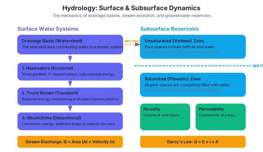
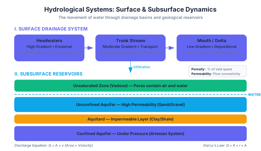
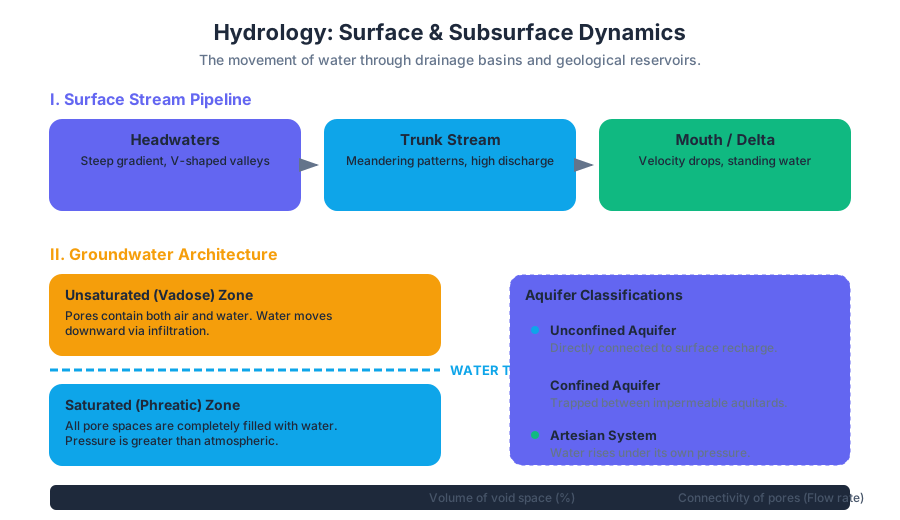
Mass Wasting and Glaciation: Mechanics of Earth in Motion

Mass wasting and glaciation represent the primary terrestrial mechanisms for the large-scale transport of lithospheric material. While driven by different physical states—one by the gravitational failure of unconsolidated or fractured rock, the other by the plastic flow of crystalline H₂O—both processes are governed by the fundamental interplay of shear stress and shear strength. In the context of a changing climate, understanding these systems is not merely a geomorphological exercise but a critical engineering necessity for hazard mitigation and resource management.

The Physics of Slope Stability

Mass wasting is the downslope movement of rock, regolith, and soil under the direct influence of gravity. Unlike erosion driven by water, wind, or ice, mass wasting does not require a transporting medium, though water often acts as a primary catalyst.

The Factor of Safety ($F_s$)

To evaluate the stability of any geological slope, engineers use the Factor of Safety, a dimensionless ratio of resisting forces to driving forces.

Definition: The Factor of Safety ($F_s$) is defined as $F_s = \frac{\sum \text{Resisting Forces}}{\sum \text{Driving Forces}}$.

• If $F_s > 1.0$, the slope is theoretically stable.
• If $F_s \leq 1.0$, the slope is in a state of failure or incipient failure.

The resisting force is primarily the shear strength ($\tau_f$) of the material, governed by the Mohr-Coulomb failure criterion: $$\tau_f = c + \sigma' \tan(\phi)$$ Where:

• $c$ is cohesion (interparticle bonding).
• $\sigma'$ is effective normal stress ($\sigma - u$, where $u$ is pore-water pressure).
• $\phi$ is the angle of internal friction.

Parameters Influencing Stability

The stability of a slope is a dynamic equilibrium influenced by several key variables:

Parameter	Impact on Stability	Physical Mechanism
Slope Angle	Decreases stability	Increases the tangential component of gravity ($G_t$).
Water Content	Decreases stability	Increases pore pressure ($u$), reducing effective stress ($\sigma'$); adds weight.
Vegetation	Increases stability	Root systems provide "apparent cohesion"; evapotranspiration removes water.
Lithology	Variable	Bedding planes dipping parallel to the slope create daylighting structures prone to failure.
Seismicity	Decreases stability	Dynamic loading creates transient increases in shear stress and liquefaction potential.

Mechanics of Mass Wasting Events

Mass wasting events are classified based on the type of material (rock vs. debris) and the type of motion (fall, slide, or flow).

Falls and Avalanches

Rockfalls occur when material detaches from a steep cliff along joints or bedding planes. Debris avalanches are higher-velocity events often triggered by volcanic eruptions or massive structural failures, characterized by air-cushioning or fluidization that allows for extreme run-out distances.

Slides: Rotational vs. Translational

1. Slumps (Rotational Slides): Movement occurs along a concave-upward curved surface. These are common in thick accumulations of cohesive soils or weak sedimentary rocks. They often result in "stair-step" topography.
2. Translational Slides: Movement occurs along a planar surface, such as a bedding plane, fault, or joint. These are often more dangerous because they can maintain structural integrity while accelerating to high speeds.

Flows and Creep

Debris flows (including lahars) behave as non-Newtonian fluids. They are mixtures of water, sediment, and air. Creep is the imperceptibly slow downslope movement of soil and regolith, driven by freeze-thaw cycles and wetting-drying cycles.

Worked Example: Infinite Slope Stability Analysis

In this low-level implementation, we calculate the Factor of Safety for a translational slide using the infinite slope model, accounting for the effect of the water table.

import numpy as np

def calculate_factor_of_safety(gamma_s, gamma_w, h, alpha, phi, cohesion, hw):
    """
    Calculates the Factor of Safety (Fs) for an infinite slope.
    
    Parameters:
    gamma_s : float : Unit weight of soil (kN/m^3)
    gamma_w : float : Unit weight of water (9.81 kN/m^3)
    h       : float : Depth to failure plane (m)
    alpha   : float : Slope angle (degrees)
    phi     : float : Friction angle (degrees)
    cohesion: float : Cohesion (kPa)
    hw      : float : Height of water table above failure plane (m)
    """
    # Convert degrees to radians
    alpha_rad = np.radians(alpha)
    phi_rad = np.radians(phi)
    
    # Total vertical stress at failure plane
    sigma_total = gamma_s * h * np.cos(alpha_rad)
    
    # Pore water pressure
    u = gamma_w * hw * np.cos(alpha_rad)**2
    
    # Effective normal stress
    sigma_prime = (gamma_s * h - gamma_w * hw) * np.cos(alpha_rad)**2
    
    # Resisting Force (Shear Strength)
    resisting = cohesion + sigma_prime * np.tan(phi_rad)
    
    # Driving Force (Shear Stress)
    driving = gamma_s * h * np.sin(alpha_rad) * np.cos(alpha_rad)
    
    fs = resisting / driving
    return fs

# Example Case: Saturated clayey silt slope
fs_result = calculate_factor_of_safety(
    gamma_s=19.0, gamma_w=9.81, h=5.0, alpha=25.0, phi=20.0, cohesion=10.0, hw=2.0
)
print(f"Calculated Factor of Safety: {fs_result:.3f}")

Glacial Systems and Dynamics

Glaciers are massive bodies of ice that form on land from the accumulation and recrystallization of snow. They are not static; they flow under their own weight, acting as the most powerful agents of erosion on Earth.

Glacial Mass Balance

The "health" of a glacier is determined by its mass balance ($B$), the difference between accumulation (snowfall, avalanching) and ablation (melting, calving, sublimation).

$$B = \int (a - s) dt$$

Where $a$ is the accumulation rate and $s$ is the ablation rate. The Equilibrium Line Altitude (ELA) marks the boundary where accumulation equals ablation.

The Mechanics of Ice Flow: Glen’s Flow Law

Ice behaves as a poly-crystalline material that deforms plastically. The relationship between the strain rate ($\dot{\epsilon}$) and shear stress ($\tau$) is non-linear.

\dot{\epsilon} = A \tau^n

Where:

• $A$ is a temperature-dependent fluidity parameter.
• $n$ is typically assumed to be 3 for glacial ice.
• $\tau$ is the basal shear stress, calculated as $\tau = \rho g h \sin(\alpha)$.

This derivation shows that ice velocity is extremely sensitive to thickness ($h$) and slope ($\alpha$). A doubling of ice thickness can lead to a sixteen-fold increase in deformation velocity.

Glacial Erosion and Landforms

Glaciers erode via two primary mechanisms:

1. Plucking (Quarrying): Meltwater penetrates fractures in bedrock, freezes, and "extracts" blocks of rock as the glacier moves.
2. Abrasion: Rocks embedded in the base of the glacier act like sandpaper, grinding the bedrock into rock flour and creating glacial striations.

Feature Type	Landform	Description
Erosional	U-Shaped Valley	Glaciers widen and deepen V-shaped river valleys into broad troughs.
Erosional	Cirque	Bowl-shaped depression at the head of a glacial valley.
Erosional	Arête	Sharp, knife-like ridge separating two cirques or glacial valleys.
Depositional	Moraine	Ridges of till (unsorted sediment) deposited at the margins of the ice.
Depositional	Esker	Sinuous ridge of stratified sand and gravel deposited by subglacial streams.
Depositional	Drumlin	Asymmetrical, teardrop-shaped hill of till aligned with ice flow direction.

Ice Ages and Paleoclimatology

The Earth has experienced multiple Ice Ages (Glacial Periods) interspersed with Interglacials. We are currently in an interglacial period of the Quaternary Ice Age.

Milankovitch Cycles

The primary drivers of long-term climate oscillation are orbital variations that change the distribution of solar radiation (insolation) reaching Earth:

• Eccentricity (100k years): The shape of Earth's orbit around the sun.
• Obliquity (41k years): The tilt of Earth's axis.
• Precession (23k years): The "wobble" of Earth's axis.

Isostatic Rebound

The massive weight of continental ice sheets (e.g., the Laurentide Ice Sheet) depresses the Earth's crust into the plastic asthenosphere. When the ice melts, the crust undergoes post-glacial isostatic rebound. This process is still occurring today in regions like Hudson Bay and Scandinavia, where the land is rising at rates of several millimeters per year.

Analyzing Glacial Retreat with Geospatial Tools

Modern glaciology relies on remote sensing. Below is a conceptual CLI workflow for processing satellite imagery to calculate the retreat of a glacier terminus.

# 1. Clip the multi-temporal satellite imagery to the glacier extent
gdalwarp -cutline glacier_bounds.shp -crop_to_cutline landsat_2000.tif landsat_2000_clipped.tif
gdalwarp -cutline glacier_bounds.shp -crop_to_cutline landsat_2023.tif landsat_2023_clipped.tif

# 2. Calculate the Normalized Difference Snow Index (NDSI)
# NDSI = (Green - SWIR) / (Green + SWIR)
gdal_calc.py -A landsat_2023_B3.tif -B landsat_2023_B6.tif \
             --outfile=ndsi_2023.tif \
             --calc="(A-B)/(A+B)"

# 3. Reclassify NDSI to create a binary mask (Ice vs. Non-Ice)
# Thresholding at 0.4 is common for snow/ice detection
gdal_calc.py -A ndsi_2023.tif --outfile=ice_mask_2023.tif --calc="A>0.4"

# 4. Compare masks to calculate area loss in square kilometers
python calculate_area_delta.py ice_mask_2000.tif ice_mask_2023.tif

Permafrost and the Cryosphere

Permafrost is defined as ground (soil or rock, including ice or organic material) that remains at or below 0°C for at least two consecutive years. It covers approximately 25% of the Northern Hemisphere's land surface.

The Thermal Regime

Permafrost consists of two main layers:

1. Active Layer: The top layer that thaws in summer and freezes in winter.
2. Permafrost Table: The upper boundary of the permanently frozen ground.

As the climate warms, the active layer deepens, leading to thermokarst—a landscape characterized by irregular surfaces of marshy hollows and small lakes formed as ice-rich permafrost thaws.

Solifluction

In permafrost regions, a specific type of mass wasting called solifluction occurs. During the summer thaw, the active layer becomes saturated with water because the underlying permafrost acts as an impermeable barrier (aquiclude). This water-logged soil flows slowly downslope even on very gentle gradients, creating lobate landforms.

Permafrost Zone	Coverage %	Typical Thickness
Continuous	90–100%	100m to 1500m
Discontinuous	50–90%	10m to 50m
Sporadic	10–50%	< 10m
Isolated Patches	< 10%	Highly localized

Common Pitfalls in Engineering and Interpretation

1. The "Water as Lubricant" Myth: While water can act as a lubricant, its primary role in mass wasting is the reduction of effective stress through pore-pressure increase. It is a hydraulic effect, not just a mechanical one.
2. Confusing Till and Outwash: Till is deposited directly by ice and is unsorted and unstratified. Outwash is deposited by meltwater and is sorted and stratified. Identifying the difference is crucial for hydrogeological modeling.
3. Ignoring Paraglacial Effects: Many landslides in mountainous regions are "paraglacial"—they are triggered by the removal of the lateral support previously provided by a glacier (buttressing). As glaciers retreat, the frequency of rockslides often increases.

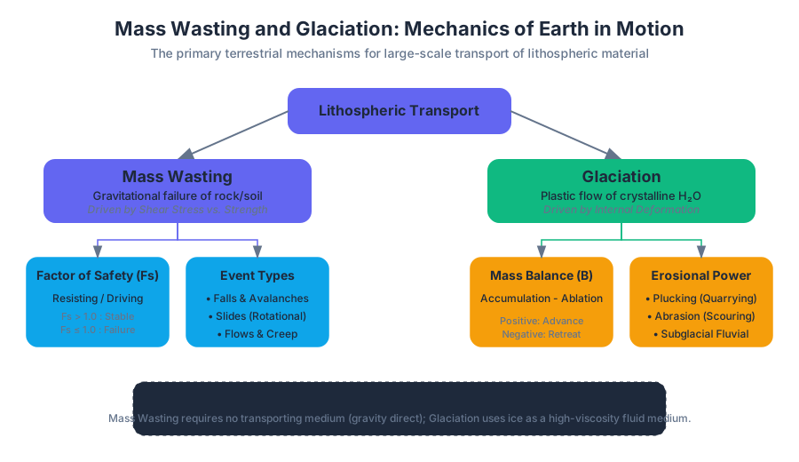
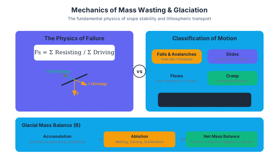
Geology of the Oceans and Shorelines

The Earth is fundamentally a marine planet, with approximately 71% of its surface submerged beneath the global ocean. From a geological perspective, the ocean floor is not merely a flooded version of the continents but a distinct tectonic and petrological regime characterized by thinner, denser basaltic crust. The study of the Geology of the Oceans and Shorelines encompasses the structural evolution of ocean basins, the sedimentological dynamics of the deep sea, and the high-energy interface where terrestrial and marine processes collide.

Understanding this domain requires a synthesis of plate tectonics, fluid dynamics, and historical geology. As sea levels fluctuate due to climatic and tectonic drivers, the boundary between land and sea—the shoreline—becomes one of the most geologically volatile environments on Earth.

Continental Margins: The Transition Zones

The Continental Margin is the submerged outer edge of a continent, representing the transition zone between thick, buoyant continental crust (primarily granitic) and thin, dense oceanic crust (primarily basaltic). These margins are categorized based on their proximity to active plate boundaries.

Passive vs. Active Margins

The distinction between passive and active margins is fundamental to understanding coastal morphology and seismic risk.

• Passive Margins: Located far from active plate boundaries (e.g., the Atlantic coast of North America). They are characterized by wide continental shelves, thick accumulations of sedimentary "clastic wedges," and low tectonic activity.
• Active Margins: Located at or near plate boundaries, typically subduction zones (e.g., the Pacific coast of South America). They feature narrow shelves, steep slopes, and deep-ocean trenches.

Feature	Passive Margin	Active Margin
Tectonic Activity	Minimal (Intraplate)	High (Subduction/Transform)
Shelf Width	Broad (up to hundreds of km)	Narrow (often < 1 km)
Trench Presence	Absent	Common (Deep-ocean trenches)
Sedimentation	High (Deltaic and Pelagic)	Variable (often scraped into accretionary prisms)
Example	East Coast, USA	West Coast, South America

Structural Components of the Margin

1. Continental Shelf: A gently sloping, submerged surface extending from the shoreline toward the deep-ocean basin. It is geologically part of the continent.
2. Continental Slope: A relatively steep structure that marks the boundary between continental and oceanic crust.
3. Continental Rise: Found only at passive margins, this is a wedge of sediment deposited at the base of the slope by turbidity currents.
4. Submarine Canyons: Deep, V-shaped valleys carved into the slope and shelf, often by ancient rivers during periods of lower sea level or by modern underwater landslides.

Definition: Turbidity Currents Dense, sediment-laden flows of water that move down the continental slope under the influence of gravity. These currents act as underwater "avalanches," transporting massive volumes of terrestrial sediment to the deep ocean floor, forming submarine fans.

The Deep Ocean Floor: Abyssal Plains and Ridges

Beyond the continental rise lies the deep-ocean basin, a realm of extreme pressure, low temperature, and unique geological features.

Abyssal Plains

The Abyssal Plains are arguably the flattest places on Earth. These vast, level areas of the deep-ocean floor result from the slow accumulation of fine-grained sediments (pelagic rain) that blanket the rugged underlying basaltic crust.

• Composition: Primarily biogenous ooze (shells of microscopic organisms) and terrigenous clay (fine dust blown from land or carried by currents).
• Significance: They serve as the ultimate "sink" for Earth's surface materials and provide a record of long-term climatic shifts.

Mid-Ocean Ridges (MORs)

The MOR system is a continuous underwater mountain range, extending over 65,000 km. It is the site of seafloor spreading, where new oceanic lithosphere is created.

Deep-Ocean Trenches

Trenches are the deepest parts of the ocean, formed at convergent plate boundaries where one lithospheric plate is subducted beneath another. The Mariana Trench, reaching depths of approximately 11,000 meters, is the most prominent example.

Ocean Feature	Typical Depth (m)	Geological Origin
Continental Shelf	0 – 200	Submerged continental crust
Abyssal Plain	3,000 – 6,000	Sediment-covered oceanic crust
Mid-Ocean Ridge	2,000 – 3,000	Divergent boundary volcanism
Ocean Trench	7,000 – 11,000	Subduction zone flexure

Coastal Dynamics: Tides and Waves

The shoreline is shaped by the continuous application of energy from the ocean, primarily in the form of waves and tides.

The Physics of Waves

Most ocean waves are generated by wind. The energy of a wave moves forward, but the water molecules themselves move in a circular orbital motion.

• Wave Base: The depth below which there is no wave-induced water movement. It is equal to approximately half the wavelength ($L/2$).
• Wave Refraction: The bending of waves as they approach the shore at an angle. Because waves slow down in shallower water, the part of the wave in deeper water "catches up," causing the wave front to become nearly parallel to the shoreline.

# Wave Physics Implementation: Calculating Wave Celerity (Speed)
# Celerity depends on water depth (d) and wavelength (L)

import math

def calculate_wave_celerity(depth, wavelength):
    """
    Calculates the speed (celerity) of a wave.
    In deep water (d > L/2), celerity depends on wavelength.
    In shallow water (d < L/20), celerity depends on depth.
    """
    g = 9.81  # Gravity m/s^2
    
    if depth > (wavelength / 2):
        # Deep water wave formula
        celerity = math.sqrt((g * wavelength) / (2 * math.pi))
        category = "Deep Water Wave"
    elif depth < (wavelength / 20):
        # Shallow water wave formula
        celerity = math.sqrt(g * depth)
        category = "Shallow Water Wave"
    else:
        # Intermediate water
        celerity = math.sqrt((g * wavelength / (2 * math.pi)) * math.tanh(2 * math.pi * depth / wavelength))
        category = "Intermediate Wave"
        
    return celerity, category

# Example: A wave with 100m wavelength in 10m of water
speed, cat = calculate_wave_celerity(10, 100)
print(f"Wave Speed: {speed:.2f} m/s | Category: {cat}")

Tides: The Gravitational Pulse

Tides are periodic rises and falls in sea level caused by the gravitational pull of the Moon and Sun.

• Spring Tides: Occur when the Sun and Moon are aligned (New/Full Moon), resulting in the highest tidal range.
• Neap Tides: Occur when the Sun and Moon are at right angles (First/Third Quarter Moon), resulting in the lowest tidal range.

Coastal Erosion and Landforms

The interaction between wave energy and the shoreline produces distinct erosional and depositional features.

Erosional Landforms

Common on active margins or rocky coastlines where wave energy is concentrated on headlands through refraction.

• Wave-cut Cliffs: Formed by the cutting action of waves at the base of a cliff.
• Sea Arches and Stacks: Formed when headlands are eroded through, leaving isolated pillars of rock.

Depositional Landforms

Common on passive margins where sediment supply exceeds the rate of removal.

• Spits: Elongated ridges of sand that project from the land into the mouth of an adjacent bay.
• Barrier Islands: Low ridges of sand that parallel the coast at distances from 3 to 30 km offshore.
• Longshore Drift: The movement of sediment along the beach in a zigzag pattern caused by waves hitting the shore at an oblique angle.

\text{Longshore Transport Rate (Q)} \approx K \cdot P_l
\\
\text{where } P_l = \text{Longshore component of wave power}
\\
K = \text{Dimensionless coefficient related to sediment characteristics}

Landform	Type	Description
Sea Stack	Erosional	Isolated rock pillar left after a sea arch collapses.
Tombolo	Depositional	A ridge of sand connecting an island to the mainland.
Estuary	Mixed	Drowned river valley where freshwater meets saltwater.
Marine Terrace	Erosional	A wave-cut platform uplifted above sea level by tectonics.

Sea Level Change: Eustasy and Isostasy

Sea level is not constant; it is a dynamic baseline that responds to global and regional factors.

1. Eustatic Sea Level Change

Global changes in sea level related to the total volume of water in the ocean or the shape of the ocean basins.

• Glacial-Interglacial Cycles: During ice ages, water is trapped on land as ice, lowering sea levels by up to 120 meters.
• Tectonic Volume Changes: Rapid seafloor spreading creates "fat" mid-ocean ridges that displace water upward, raising sea levels.

2. Relative Sea Level Change

Local changes caused by the movement of the land itself.

• Isostatic Rebound: Land that was once depressed by the weight of glaciers rises after the ice melts (e.g., Scandinavia, Hudson Bay).
• Subsidence: Land sinking due to sediment loading or groundwater extraction (e.g., New Orleans, Venice).

Key Insight: Transgression vs. Regression A Transgression occurs when sea level rises relative to the land, moving the shoreline inland. A Regression occurs when sea level falls, exposing the former seafloor. These events are recorded in the rock record as specific vertical sequences of sedimentary facies.

Human Interaction and Coastal Engineering

As humans inhabit coastal zones, we attempt to stabilize dynamic shorelines using engineering structures. However, these often have unintended geological consequences.

Stabilization Structures

1. Jetties: Built in pairs at the entrances to harbors to prevent sedimentation.
2. Groins: Short walls built perpendicular to the shore to trap sand moving via longshore drift.
3. Seawalls: Massive barriers built parallel to the shore to protect property from breaking waves.
4. Breakwaters: Offshore barriers built parallel to the coast to create quiet water zones.

The "Sand Deficit" Problem

Groins and jetties trap sand on the "up-drift" side but cause accelerated erosion on the "down-drift" side because the longshore current is "starved" of sediment.

# Example: Fetching Coastal Erosion Data (Hypothetical CLI Tool)
# Engineers use NOAA/USGS APIs to monitor shoreline retreat rates.

$ coastal-tool fetch --station-id 8443970 --start-date 2020-01-01 --end-date 2023-12-31
$ coastal-tool analyze-erosion --input shoreline_data.json --threshold 0.5

# Output:
# [INFO] Analyzing Station 8443970 (Boston, MA)
# [WARN] Annual Retreat Rate: 0.72m/year exceeds safety threshold (0.5m/year)
# [INFO] Recommendation: Beach nourishment required for Sector 4.

Common Pitfalls in Marine Geology

• Misunderstanding Wave Motion: A common mistake is thinking water moves forward with a wave in the open ocean. In reality, only the energy moves forward; the water particles return to nearly the same spot.
• Passive Margin = No Change: While "passive" implies no plate boundary, these margins are still dynamic. They experience massive sediment loading, salt tectonics, and significant sea-level fluctuations.
• The "Static Shoreline" Fallacy: Many coastal developments are built on the assumption that the shoreline is a fixed line. Geologically, the shoreline is a migrating feature that responds to every storm and every millimeter of sea-level rise.

-- Database Schema for Coastal Monitoring
CREATE TABLE ShorelineObservations (
    observation_id INT PRIMARY KEY,
    location_coord GEOGRAPHY,
    date_observed DATE,
    mean_high_water_mark FLOAT, -- meters relative to datum
    sediment_type VARCHAR(50),
    erosion_rate_annual FLOAT    -- calculated mm/year
);

-- Query to find high-risk erosion zones
SELECT location_coord, erosion_rate_annual
FROM ShorelineObservations
WHERE erosion_rate_annual > 10.0
ORDER BY erosion_rate_annual DESC;

Summary of Key Concepts

1. Continental Margins define the edge of the continental block; passive margins are stable and wide, while active margins are narrow and tectonically volatile.
2. Abyssal Plains are the result of millions of years of fine-grained sedimentation covering the volcanic topography of the ocean floor.
3. Waves and Tides are the primary drivers of coastal change, with wave refraction focusing energy on headlands and longshore drift moving sediment like a conveyor belt.
4. Sea Level is a function of both global water volume (eustasy) and local land movement (isostasy).
5. Human Engineering often disrupts the natural "sand budget" of a coastline, leading to unintended erosion in adjacent areas.

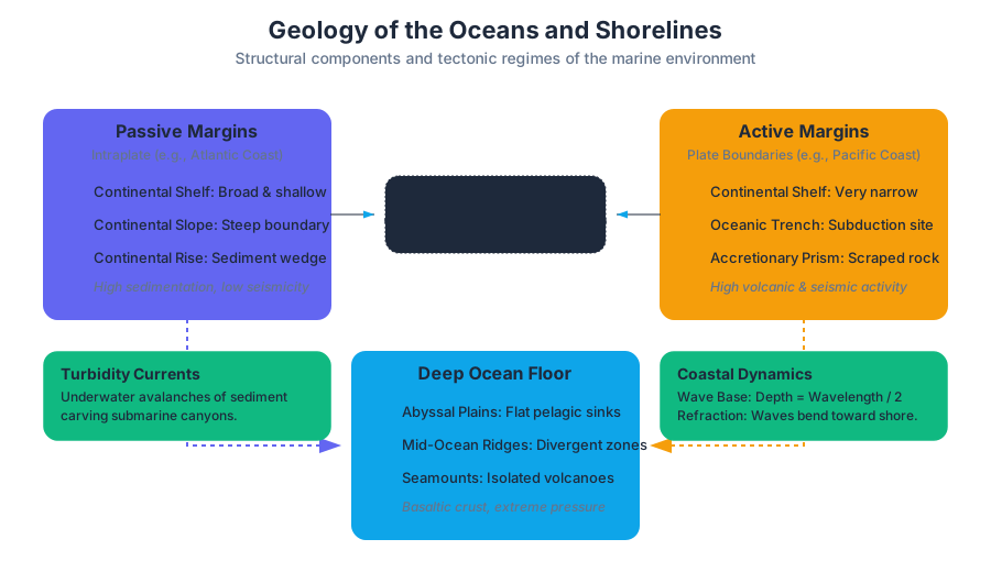
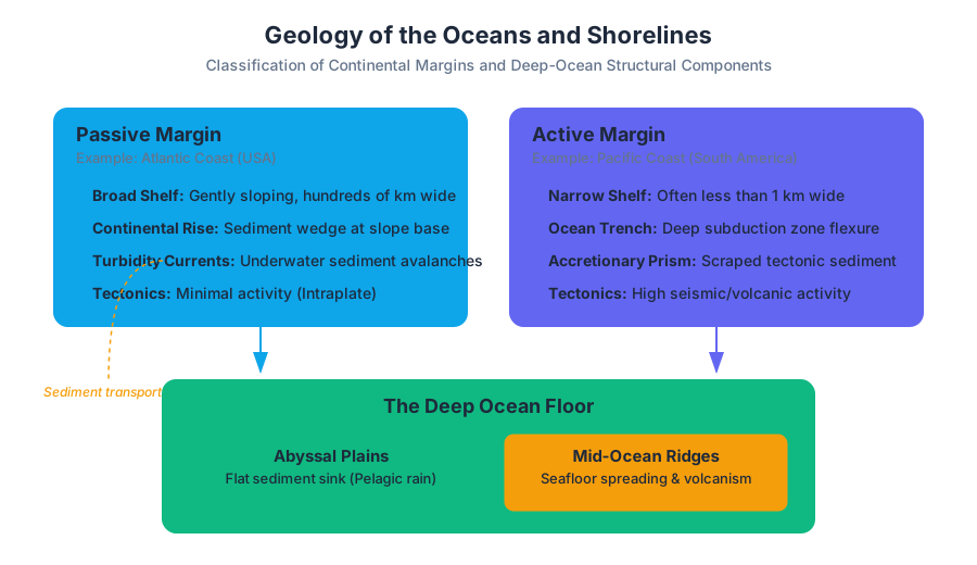
Climate Change and Environmental Geology

Earth System Science (ESS)

Earth System Science is the study of the Earth as a complex, integrated system of interacting physical, chemical, and biological processes. Unlike traditional geology, which may focus solely on the lithosphere, ESS treats the planet as a synergistic whole where the transfer of energy and matter occurs across several "spheres."

Definition: The Earth System is composed of the Atmosphere (air), Hydrosphere (water), Cryosphere (ice), Biosphere (life), and Geosphere (solid earth). These components are linked through biogeochemical cycles and feedback loops that regulate the planet's state.

The Dynamics of Feedback Loops

In environmental geology, we distinguish between two primary types of feedback mechanisms:

1. Positive Feedback: A process where the initial change is amplified by the system's response. For example, the Ice-Albedo Feedback: as temperatures rise, ice melts, reducing the Earth's reflectivity (albedo), causing further warming.
2. Negative Feedback: A process where the system responds in a way that reverses or dampens the initial change, promoting stability. For example, increased $CO_2$ can lead to enhanced plant growth (the "greening" effect), which subsequently removes $CO_2$ from the atmosphere.

Sphere	Primary Function in Climate	Typical Residence Time
Atmosphere	Heat transport and greenhouse insulation	Days to Weeks (for water vapor)
Hydrosphere	Thermal inertia and $CO_2$ absorption	100s to 1000s of years (Deep Ocean)
Cryosphere	Albedo regulation and sea-level storage	10s to 100,000s of years
Geosphere	Long-term carbon sequestration (silicate weathering)	Millions of years
Biosphere	Rapid carbon cycling and methane production	Decades to Centuries

The Greenhouse Effect and Radiative Forcing

The Greenhouse Effect is the process by which certain gases in the atmosphere absorb and re-emit infrared radiation, effectively trapping heat. Without this natural process, Earth's average surface temperature would be approximately -18°C (0°F), rather than the current hospitable 15°C (59°F).

The Physics of Radiative Balance

The Earth's temperature is determined by the balance between incoming solar radiation (shortwave) and outgoing terrestrial radiation (longwave). This is governed by the Stefan-Boltzmann Law:

$$P = \sigma A T^4$$

Where:

• $P$ is the power radiated.
• $\sigma$ is the Stefan-Boltzmann constant ($5.67 \times 10^{-8} W m^{-2} K^{-4}$).
• $A$ is the surface area.
• $T$ is the absolute temperature in Kelvin.

Greenhouse Gas (GHG) Efficiency

Not all gases are created equal. Their impact is measured by Global Warming Potential (GWP), which compares the heat-trapping ability of a gas relative to $CO_2$ over a specific timeframe (usually 100 years).

Greenhouse Gas	Formula	GWP (100-yr)	Atmospheric Lifetime
Carbon Dioxide	$CO_2$	1	50–200 years
Methane	$CH_4$	28–36	~12 years
Nitrous Oxide	$N_2O$	265–298	~114 years
Chlorofluorocarbons	CFC-11	4,660	~45 years

Implementation: Calculating Radiative Equilibrium

The following Python implementation calculates the theoretical "Blackbody" temperature of Earth versus the observed temperature, illustrating the magnitude of the Greenhouse Effect.

import math

def calculate_earth_temp(solar_constant, albedo):
    """
    Calculates the effective emission temperature of Earth (K).
    Formula: T = ((S * (1 - alpha)) / (4 * sigma))^(1/4)
    """
    SIGMA = 5.670374419e-8  # Stefan-Boltzmann constant
    
    # Calculate absorbed flux
    absorbed_flux = (solar_constant * (1 - albedo)) / 4
    
    # Solve for T
    temperature_kelvin = math.pow(absorbed_flux / SIGMA, 0.25)
    
    return temperature_kelvin

# Constants for Earth
S_EARTH = 1361  # W/m^2 (Solar Constant)
ALBEDO_EARTH = 0.30

temp_k = calculate_earth_temp(S_EARTH, ALBEDO_EARTH)
temp_c = temp_k - 273.15

print(f"Theoretical Blackbody Temp: {temp_k:.2f} K ({temp_c:.2f} °C)")
# Output: Theoretical Blackbody Temp: 254.62 K (-18.53 °C)

Paleoclimatology: The Geologic Record

Paleoclimatology is the study of past climates. Because instrumental records only exist for the last ~150 years, geologists use proxies—physical, chemical, or biological signatures preserved in the geologic record—to reconstruct Earth's history.

Isotopic Fractionation ($\delta^{18}O$)

The most critical tool in paleoclimatology is the ratio of stable oxygen isotopes, $^{18}O$ and $^{16}O$.

• $^{16}O$ is lighter and evaporates more easily.
• $^{18}O$ is heavier and condenses more readily.

During glacial periods, $^{16}O$ is trapped in ice sheets on land, leaving the ocean enriched in $^{18}O$. Therefore, high $\delta^{18}O$ values in the calcium carbonate ($CaCO_3$) shells of marine foraminifera indicate colder global temperatures and higher ice volume.

Derivation of the Delta Notation

The "delta" value is a way to express small variations in isotopic ratios relative to a standard (usually V-SMOW or PDB).

\delta^{18}O = \left( \frac{(^{18}O/^{16}O)_{sample}}{(^{18}O/^{16}O)_{standard}} - 1 \right) \times 1000 \text{ ‰}

Paleoclimate Proxies and Their Utility

Proxy Type	Resolution	Time Range	Climate Information
Ice Cores	Annual	< 800,000 years	Gas composition ($CO_2$, $CH_4$), Temp
Tree Rings	Annual	< 10,000 years	Precipitation, Local Temp
Marine Sediments	Decadal/Centennial	< 100 Million years	Global ice volume, Ocean temp
Speleothems	Annual/Decadal	< 500,000 years	Groundwater chemistry, Rainfall

Milankovitch Cycles: The Orbital Pacemaker

Long-term natural climate variability is driven by predictable changes in Earth's orbit, known as Milankovitch Cycles. These cycles alter the seasonal and latitudinal distribution of solar radiation (insolation).

1. Eccentricity (~100,000 years): The shape of Earth's orbit changes from nearly circular to mildly elliptical. This affects the total amount of radiation received at different times of the year.
2. Obliquity (~41,000 years): The tilt of Earth's axis varies between 22.1° and 24.5°. A higher tilt increases seasonal contrast, particularly at the poles.
3. Precession (~23,000 years): The "wobble" of Earth's axis. This determines which hemisphere is tilted toward the sun during perihelion (closest approach).

Key Insight: Glaciation is typically triggered not by cold winters, but by cool summers in the Northern Hemisphere. If summer insolation is low enough, the previous winter's snow does not melt, allowing ice sheets to grow.

Data Structure for Orbital Forcing

In computational geology, we often handle these cycles as time-series data to force climate models.

# Orbital Parameters for a Paleoclimate Simulation (Simplified)
simulation_metadata:
  target_era: "Last Glacial Maximum"
  years_bp: 21000
orbital_parameters:
  eccentricity: 0.018994
  obliquity_degrees: 22.949
  precession_longitude_of_perihelion: 114.42
boundary_conditions:
  co2_ppm: 190
  ch4_ppb: 375
  ice_sheet_extent: "Laurentide_Max"

Anthropogenic Impact and the Carbon Cycle

While natural cycles operate over millennia, the Anthropogenic Impact refers to the rapid changes induced by human activity since the Industrial Revolution. The primary driver is the perturbation of the Carbon Cycle.

The Short-Term vs. Long-Term Carbon Cycle

• Short-Term: Movement of carbon between the atmosphere, biosphere, and upper ocean. Fluxes are large and rapid.
• Long-Term (Geologic): Movement of carbon into and out of the lithosphere via subduction, volcanism, and silicate weathering.

Silicate Weathering: The Earth's Thermostat

The Earth has a natural "brake" on warming called the Urey Reaction. Increased temperatures and rainfall accelerate the weathering of silicate rocks, which consumes $CO_2$:

CaSiO_3 + CO_2 \rightarrow CaCO_3 + SiO_2

The resulting calcium carbonate is washed into the oceans and buried as limestone. This process takes hundreds of thousands of years—far too slow to mitigate current human emissions.

Environmental Geology and Natural Hazards

Climate change acts as a "threat multiplier" for geological hazards. As the energy balance of the Earth changes, the frequency and intensity of surface processes shift.

1. Hydrological Hazards

Increased global temperatures lead to a more vigorous hydrological cycle. For every 1°C of warming, the atmosphere can hold approximately 7% more water vapor (the Clausius-Clapeyron relationship).

• Flooding: Increased high-intensity rainfall events overwhelm drainage basins.
• Drought: Enhanced evaporation depletes soil moisture and groundwater.

2. Mass Wasting (Landslides)

In mountainous regions, the melting of permafrost (permanently frozen ground) destabilizes slopes. Additionally, extreme precipitation events increase pore-water pressure in soil, triggering debris flows and landslides.

3. Coastal Erosion and Sea-Level Rise

Sea-level rise is driven by two factors:

• Thermal Expansion: As water warms, it expands.
• Eustatic Change: The melting of land-based ice (glaciers and ice sheets) adds volume to the ocean.

Hazard	Climate Link	Geological Impact
Landslides	Increased precipitation intensity	Slope failure, loss of regolith
Coastal Erosion	Sea-level rise + Storm surges	Retrogradation of shorelines
Subsidence	Groundwater over-extraction (drought)	Permanent loss of aquifer porosity
Glacial Lake Outbursts	Rapid glacial retreat	Catastrophic downstream flooding

Example: Processing Sea Level Data

A senior geologist might use a shell pipeline to extract and summarize sea-level anomaly data from a global monitoring station.

# Extracting mean sea level (MSL) anomalies from a CSV dataset
# Column 1: Date, Column 12: MSL Anomaly (mm)

grep -v '^#' sea_level_data.csv | \
awk -F',' '{sum+=$12; count++} END {print "Average Anomaly: " sum/count " mm"}'

# Output: Average Anomaly: 98.42 mm

Scientific Consensus and Modeling

The consensus on anthropogenic climate change is built upon multiple independent lines of evidence:

1. Direct Measurements: The Keeling Curve (atmospheric $CO_2$ at Mauna Loa).
2. Fingerprinting: Observed warming patterns match the "signature" of greenhouse warming (e.g., a cooling stratosphere while the troposphere warms).
3. Numerical Models: General Circulation Models (GCMs) cannot replicate the observed 20th-century warming using only natural forcings (solar and volcanic). They only match observations when human-produced GHGs are included.

Common Pitfalls in Interpretation

• Confusing Weather with Climate: Weather is the state of the atmosphere at a specific moment; climate is the long-term statistical average (usually 30 years).
• The "Hiatus" Myth: Short-term plateaus in surface temperature are often due to heat being sequestered in the deep ocean, not a cessation of global warming.
• Solar Misconception: While the Sun varies on an 11-year cycle, solar irradiance has actually trended slightly downward since the 1960s, while temperatures have soared.

Summary of Environmental Management

Geologists play a crucial role in Climate Adaptation and Mitigation:

• Carbon Capture and Sequestration (CCS): Injecting $CO_2$ into depleted oil reservoirs or saline aquifers.
• Resource Management: Mapping shifting groundwater resources as recharge patterns change.
• Hazard Mapping: Redefining 100-year floodplains in response to a non-stationary climate.

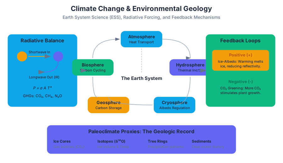
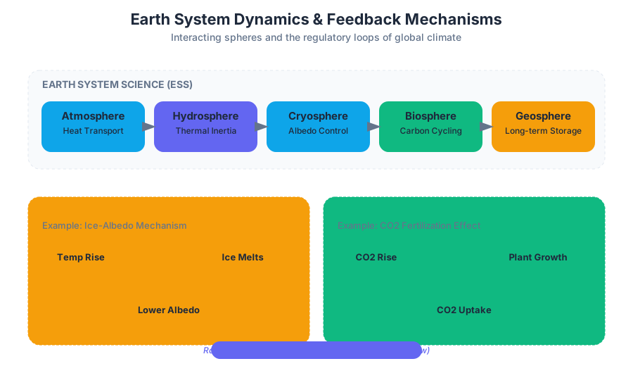
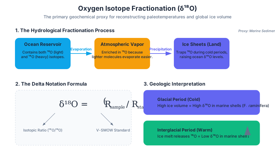
Geological Resources and Energy

The study of geological resources and energy is the study of how the Earth’s lithosphere acts as both a battery and a warehouse for human civilization. From the concentrated chemical energy of hydrocarbons to the structural utility of rare-earth minerals, the extraction and management of these resources define the boundaries of modern economic and technological capability. This section explores the formation, quantification, and socio-technical challenges of harnessing Earth's materials.

Fossil Fuels: The Hydrocarbon Ledger

Fossil fuels are concentrated solar energy stored in the form of organic carbon. Over millions of years, biological productivity in the oceans and terrestrial swamps is preserved in sedimentary basins, undergoing chemical transformation under increasing pressure and temperature.

The Formation Pipeline: Diagenesis to Metagenesis

The transformation of organic matter into fuel follows a specific thermal trajectory. The primary precursor is kerogen, a solid, waxy organic substance.

1. Diagenesis: Occurs at shallow depths and low temperatures (< 50°C). Microbial activity breaks down organic matter into biogenic methane.
2. Catagenesis: The "Oil Window" (approx. 60°C to 120°C). Kerogen cracks into liquid hydrocarbons.
3. Metagenesis: The "Gas Window" (120°C to 200°C). Liquid hydrocarbons break down into dry natural gas (methane).

The Oil Window Principle: Liquid petroleum is metastable. If a source rock is buried too deeply, the thermal energy exceeds the C-C bond strength of long-chain hydrocarbons, resulting in thermal cracking into methane.

Quantitative Maturation: The Arrhenius Approach

The maturation of kerogen is a kinetic process. We can model the transformation ratio ($TR$) using the Arrhenius equation, where the rate of reaction $k$ depends on the activation energy $E_a$ and the absolute temperature $T$.

k = A \exp\left(-\frac{E_a}{RT}\right)

Where:

• $A$ is the frequency factor.
• $R$ is the universal gas constant.
• $T$ is temperature in Kelvin.

Fuel Type	Carbon Content (%)	Energy Density (MJ/kg)	Primary Environment
Peat	< 60	10–15	Swamps/Wetlands
Lignite	60–70	15–20	Shallow Burial
Bituminous	70–86	24–35	Deep Basin Burial
Anthracite	86–98	33–36	Tectonic Compression

Natural Gas Exploration and Shale Mechanics

Natural gas, particularly in "unconventional" reservoirs like shale, has redefined the global energy landscape. Unlike conventional reservoirs where gas migrates into a porous sandstone "trap," shale gas remains locked within the source rock itself.

Porosity vs. Permeability

In shale exploration, the challenge is not the volume of gas (porosity) but the ability of the gas to flow (permeability). Shales often have high porosity but nanodarcy-level permeability.

To extract this gas, engineers use Hydraulic Fracturing (fracking). By injecting high-pressure fluid, the rock is induced to fail in tension, creating a network of artificial fractures.

Implementation: Simulating Fluid Flow in Porous Media

The following C code demonstrates a simplified 1D finite-difference solver for Darcy's Law, representing how pressure dissipates through a reservoir over time.

#include <stdio.h>

#define NX 100    // Number of spatial steps
#define NT 5000   // Number of time steps
#define DX 1.0    // Spatial step size (m)
#define DT 0.01   // Time step size (s)
#define K    1e-12 // Permeability (m^2)
#define PHI  0.2   // Porosity
#define MU   1e-3  // Viscosity (Pa*s)
#define COMP 1e-9  // Total compressibility (1/Pa)

int main() {
    double P[NX], P_new[NX];
    double alpha = K / (PHI * MU * COMP); // Diffusivity constant

    // Initialize Reservoir Pressure (Pa)
    for (int i = 0; i < NX; i++) P[i] = 2e7; 

    // Boundary Condition: Wellbore at P=1e6 at x=0
    P[0] = 1e6;

    for (int t = 0; t < NT; t++) {
        for (int i = 1; i < NX - 1; i++) {
            P_new[i] = P[i] + alpha * DT / (DX * DX) * (P[i+1] - 2*P[i] + P[i-1]);
        }
        // Update P and maintain boundary conditions
        for (int i = 1; i < NX - 1; i++) P[i] = P_new[i];
        P[0] = 1e6; 
        P[NX-1] = 2e7;
    }

    printf("Pressure at center: %e Pa\n", P[NX/2]);
    return 0;
}

Mineral Deposits: The Concentration Factor

A mineral deposit is a volume of rock where a specific element is concentrated significantly above its average crustal abundance. The economic viability of a deposit is determined by the Concentration Factor ($C_f$).

C_f = \frac{\text{Grade of Ore}}{\text{Crustal Abundance}}

For example, the average crustal abundance of Aluminum is ~8%, while Gold is ~0.0000004%. Consequently, Gold requires a much higher $C_f$ to be economically minable.

Types of Mineral Enrichment

1. Magmatic: Heavy minerals (like Chromite) settle to the bottom of a cooling magma chamber via fractional crystallization.
2. Hydrothermal: Hot, chemically active fluids dissolve metals from large volumes of rock and precipitate them in concentrated veins or "chimneys" (e.g., VMS deposits).
3. Sedimentary (Placer): Heavy, chemically resistant minerals (Gold, Diamonds) are mechanically concentrated by running water in riverbeds.

Metal	Ore Mineral	Chemical Formula	Typical Ore Grade
Iron	Hematite	$Fe_2O_3$	30–60%
Copper	Chalcopyrite	$CuFeS_2$	0.5–2.0%
Aluminum	Bauxite	$Al(OH)_3$	30–50%
Lithium	Spodumene	$LiAl(Si_2O_6)$	1–2%

Renewable Energy: The Geothermal and Mineral Nexus

Renewable energy is often framed as "clean," but it remains deeply tethered to geological resources.

Geothermal Energy

Geothermal systems exploit the Geothermal Gradient—the rate at which temperature increases with depth (averaging 25°C/km). In tectonically active areas, this gradient is much higher, allowing for the extraction of steam to drive turbines.

The "Green" Mineral Crisis

Transitioning to wind, solar, and electric vehicles (EVs) requires a massive increase in mineral extraction. A single EV battery can require 10kg of Lithium, 35kg of Nickel, and 15kg of Cobalt. This shifts the geological challenge from fuel extraction to mineral extraction.

Data Analysis: Energy Return on Investment (EROI)

The following Python snippet calculates the EROI for different energy sources, a critical metric for evaluating the long-term sustainability of a resource.

import pandas as pd

# Data: Energy delivered to society vs Energy required to get that energy
energy_data = {
    'Source': ['Coal', 'Conventional Oil', 'Shale Gas', 'Solar PV', 'Wind'],
    'Energy_Output': [80, 100, 30, 12, 20],
    'Energy_Input': [2, 3, 2, 1, 1]
}

df = pd.DataFrame(energy_data)
df['EROI'] = df['Energy_Output'] / df['Energy_Input']

# Sort by most efficient
df = df.sort_values(by='EROI', ascending=False)

print("Energy Return on Investment (EROI) Analysis:")
print(df[['Source', 'EROI']])

# Example Output:
# Source             EROI
# Conventional Oil   33.33
# Coal               40.00
# Wind               20.00
# Shale Gas          15.00
# Solar PV           12.00

Civil Dialogue: The "Marcellus Matters" Case Study

Geological resources do not exist in a vacuum; they exist beneath communities. The Marcellus Shale in the Appalachian Basin serves as a primary example of the tension between economic gain and environmental risk.

The "Marcellus Matters" Framework

"Marcellus Matters" was a project designed to foster civil dialogue regarding natural gas exploration. It moved beyond binary "pro-fracking" vs. "anti-fracking" stances by focusing on:

• Baseline Monitoring: Engaging citizens in testing their own well water before drilling begins.
• Socio-Economic Impact: Discussing "Boom-Bust" cycles and the strain on local infrastructure (roads, housing).
• Social License to Operate (SLO): The idea that companies need more than just legal permits; they need the ongoing acceptance of the local community.

The Complexity of Dialogue

Civil dialogue in geology requires translating complex subsurface uncertainties into transparent public information.

Stakeholder	Primary Concern	Geological Metric
Industry	Profitability / Flow Rate	Permeability ($k$), EUR (Estimated Ultimate Recovery)
Homeowner	Water Quality	Aquifer depth vs. Frack zone depth
Local Gov	Infrastructure	Seismic activity (Induced Seismicity), Truck traffic
Ecologist	Habitat Fragmentation	Surface footprint of well pads

Environmental Impacts and Mitigation

Resource extraction inevitably alters the environment. Understanding the geochemistry of these impacts is essential for mitigation.

Acid Mine Drainage (AMD)

When sulfide minerals (like Pyrite, $FeS_2$) are exposed to air and water during mining, they oxidize to form sulfuric acid.

The Chemical Pathway:

1. $2FeS_2 + 7O_2 + 2H_2O \rightarrow 2Fe^{2+} + 4SO_4^{2-} + 4H^+$
2. The resulting acidity ($H^+$) lowers the pH, often to levels below 3.0, leaching heavy metals into the watershed.

Land Subsidence

The removal of fluids (oil, gas, or groundwater) reduces pore pressure, causing the overlying sediment to collapse under its own weight. This is modeled using Terzaghi's Principle of Effective Stress:

\sigma' = \sigma - u

Where:

• $\sigma'$ is effective stress (grain-to-grain contact).
• $\sigma$ is total stress (overburden).
• $u$ is pore fluid pressure.

When $u$ decreases, $\sigma'$ increases, leading to compaction.

Database Management: Tracking Mineral Grades

To manage large-scale extraction, geologists use SQL databases to track ore quality across different mine sectors.

-- Query to find sectors with high-grade copper but high arsenic impurities
SELECT sector_id, copper_grade, arsenic_ppm, volume_m3
FROM mine_samples
WHERE copper_grade > 1.5 
  AND arsenic_ppm < 50
ORDER BY copper_grade DESC;

Common Pitfalls in Resource Geology

• The "Infinite Resource" Fallacy: Assuming that technological advancement will always stay ahead of depletion. While technology lowers the economic cutoff for ore, it cannot override the thermodynamic limits of extraction.
• Ignoring Scale: A common mistake is comparing the "cleanliness" of a solar panel at the point of use with a coal plant, without accounting for the geological footprint of the silver, silicon, and copper mining required for the panel.
• Correlation vs. Causation in Seismicity: Not all earthquakes near drill sites are caused by fracking. Most "induced seismicity" is actually caused by the deep-well injection of waste fluids, not the fracturing process itself.