From the free course Computing on Lykke
Simulations and Control Flow
Key concepts: Break and Continue · Randomness · Simulating natural selection
Controlling loop execution and using randomness to simulate real-world phenomena.
Simulations and Control Flow
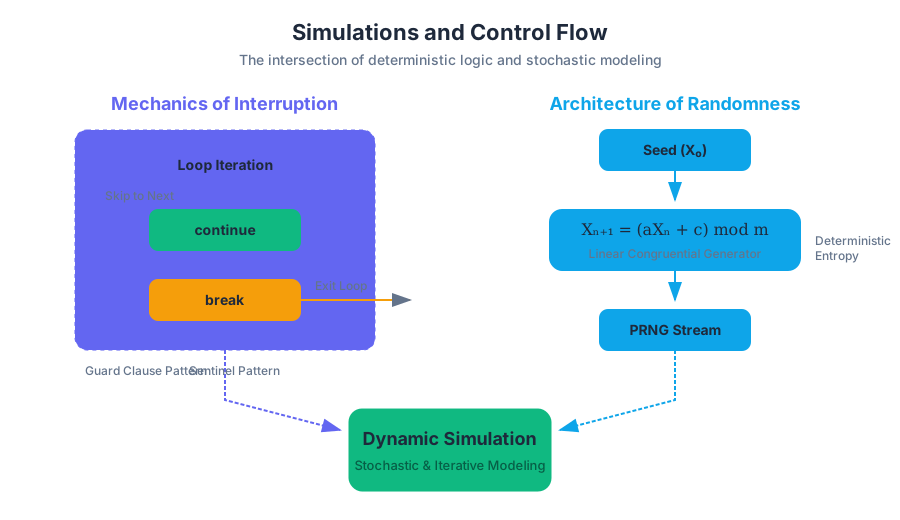
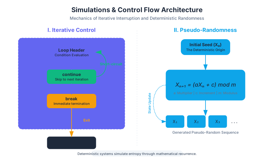
In the architecture of computational logic, the transition from static scripts to dynamic simulations represents a fundamental leap in complexity. While basic algorithms follow a linear or strictly branching path, Simulations allow us to model the stochastic (random) and iterative nature of reality. To build these models, we must master the fine-grained control of execution flow—specifically how to interrupt, skip, or terminate cycles—and how to inject controlled entropy through randomness.
This section dissects the mechanics of loop control, the mathematical foundations of pseudo-randomness, and the implementation of biological heuristics through simulated natural selection.
The Mechanics of Interruption: Break and Continue
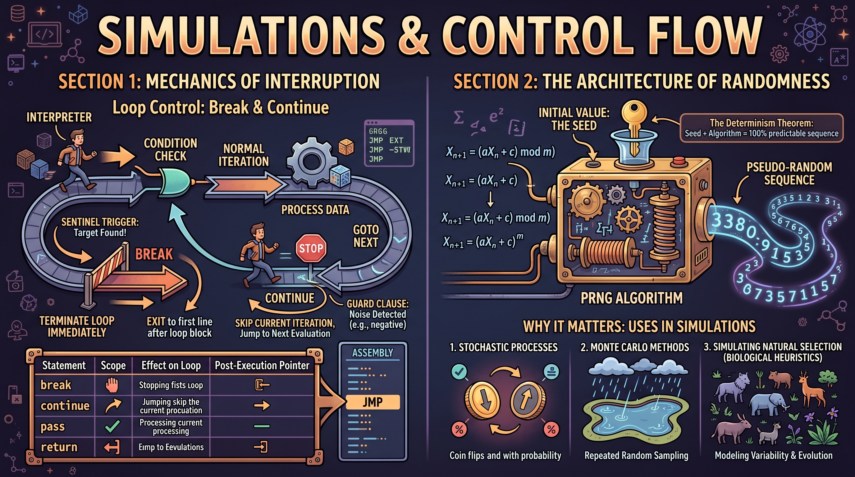
In standard iterative logic, a loop executes its block until a condition is met. However, real-world data is often "noisy" or contains early-exit triggers. To handle these, we employ non-local control flow statements: break and continue. These are not merely "shortcuts"; they are essential tools for optimizing algorithmic complexity and maintaining clean code architecture.
1. The break Statement: Immediate Termination
The break statement provides an "emergency exit" from the innermost loop. When the interpreter encounters break, it immediately halts the loop's execution and jumps to the first line of code following the loop block.
- Mathematical Motivation: In search algorithms, once the target element $x$ is found in set $S$, further iterations are $O(n)$ waste.
breakallows us to achieve an average-case performance of $O(n/2)$ rather than forcing $O(n)$. - The Sentinel Pattern:
breakis frequently used in "infinite" loops (while True) where the exit condition is complex or depends on external input that cannot be evaluated at the loop's header.
2. The continue Statement: Iterative Skipping
Unlike break, continue does not terminate the loop. Instead, it "short-circuits" the current iteration, skipping the remaining code in the block and jumping directly to the next evaluation of the loop condition (in while loops) or the next element (in for loops).
- The Guard Clause Pattern:
continueis used to avoid deeply nestedifstatements (the "Arrow Anti-pattern"). By checking for invalid data at the top of a loop and usingcontinue, the "happy path" of the code remains at a low indentation level.
| Statement | Scope | Effect on Loop | Post-Execution Pointer |
|---|---|---|---|
break |
Innermost loop | Terminates loop immediately | First line after the loop block |
continue |
Innermost loop | Skips current iteration | Next iteration/condition check |
pass |
Any block | No effect (placeholder) | Next line in the same block |
return |
Function | Terminates function | Back to the caller |
Implementation: Low-Level Control Flow in C
To understand how these work under the hood, we look at the assembly-like behavior in C, where these statements translate to JMP (jump) instructions in the CPU.
#include <stdio.h>

/**
 * Demonstrates a robust search and filter simulation.
 * We search for a target value but skip "noisy" data (negative numbers).
 */
int main() {
    int data[] = {10, -5, 20, 33, -1, 40, 50};
    int target = 33;
    int size = sizeof(data) / sizeof(data[0]);

    for (int i = 0; i < size; i++) {
        // 1. Noise Filtering (Continue)
        if (data[i] < 0) {
            printf("Skipping noise at index %d\n", i);
            continue;
        }

        // 2. Target Identification (Break)
        if (data[i] == target) {
            printf("Target %d found at index %d. Terminating search.\n", target, i);
            break;
        }

        printf("Processing valid data: %d\n", data[i]);
    }
    return 0;
}
The Architecture of Randomness
Simulations require unpredictability. However, computers are inherently deterministic machines—given the same input and state, they will always produce the same output. To simulate "randomness," we use Pseudo-Random Number Generators (PRNGs).
What it is
A PRNG is an algorithm that uses mathematical formulas to produce sequences of numbers that appear random. These sequences are actually deterministic and originate from an initial value called a Seed.
The Determinism Theorem: If you know the seed and the algorithm of a PRNG, you can predict every subsequent number in the sequence with 100% accuracy.
Why it matters
In simulations, we use randomness to model:
- Stochastic Processes: Events that have a known probability but an uncertain outcome (e.g., a coin flip).
- Monte Carlo Methods: Using repeated random sampling to obtain numerical results (e.g., calculating the area under a curve).
- Variability: Ensuring that a simulation of a forest or a population doesn't result in identical "clones."
Mathematical Derivation: The Linear Congruential Generator (LCG)
Most basic random modules (like Python's random or C's rand()) are based on variations of the LCG. The formula for generating the next number $X_{n+1}$ is:
X_{n+1} = (aX_n + c) \pmod m
Where:
- $X$ is the sequence of pseudo-random values.
- $m$ is the "modulus" (the maximum range).
- $a$ is the "multiplier."
- $c$ is the "increment."
- $X_0$ is the Seed.
| Parameter | Constraint | Purpose |
|---|---|---|
m |
$m > 0$ | Defines the period length (how long before the sequence repeats). |
a |
$0 < a < m$ | Controls the "shuffling" of bits. |
c |
$0 \le c < m$ | Ensures the sequence doesn't get stuck at zero. |
seed |
$0 \le seed < m$ | The starting point of the sequence. |
Common Pitfalls: The Seed Trap
A common mistake is re-seeding the generator inside a loop. If you set the seed to the current system time inside a fast-running loop, the time may not change between iterations, causing the "random" generator to return the exact same number repeatedly. Always seed once at the start of the program.
Simulating Natural Selection
Natural selection is the ultimate biological algorithm. It is a process where individuals with favorable traits are more likely to reproduce, passing those traits to the next generation. In computer science, we model this using Genetic Algorithms (GAs).
The Simulation Pipeline
A simulation of natural selection follows a specific iterative loop:
- Initialization: Create a population of individuals with random traits (chromosomes).
- Fitness Evaluation: Calculate a "fitness score" for each individual based on how well they solve a specific problem.
- Selection: Choose the "parents" for the next generation, favoring those with higher fitness scores.
- Crossover (Recombination): Combine traits from two parents to create offspring.
- Mutation: Randomly flip or change a trait in the offspring to maintain genetic diversity.
- Replacement: Replace the old population with the new generation and repeat.
Concrete Example: The "String Evolution" Simulation
Imagine we want to evolve a random string of characters until it matches the target phrase "EVOLVE".
- Fitness: Number of characters in the correct position.
- Mutation Rate: The probability (e.g., 1%) that a character changes randomly.
Implementation: Python Population Simulation
This example uses a high-level approach to model a population evolving toward a target.
import random

# Configuration
TARGET = "EVOLVE"
ALPHABET = "ABCDEFGHIJKLMNOPQRSTUVWXYZ "
POP_SIZE = 100
MUTATION_RATE = 0.01

def get_fitness(genome):
    """Calculates how many characters match the target."""
    return sum(1 for g, t in zip(genome, TARGET) if g == t)

def mutate(genome):
    """Randomly alters a gene based on the mutation rate."""
    genome_list = list(genome)
    for i in range(len(genome_list)):
        if random.random() < MUTATION_RATE:
            genome_list[i] = random.choice(ALPHABET)
    return "".join(genome_list)

# 1. Initialization
population = ["".join(random.choice(ALPHABET) for _ in range(len(TARGET)))
              for _ in range(POP_SIZE)]

generation = 0
while True:
    generation += 1

    # 2. Evaluation & Selection (Sort by fitness)
    population.sort(key=get_fitness, reverse=True)
    best_individual = population[0]

    if get_fitness(best_individual) == len(TARGET):
        print(f"Gen {generation}: {best_individual} (Target Reached!)")
        break

    if generation % 10 == 0:
        print(f"Gen {generation}: {best_individual} | Fitness: {get_fitness(best_individual)}")

    # 3. Reproduction (Top 10% survive and breed)
    new_population = population[:10]
    while len(new_population) < POP_SIZE:
        parent = random.choice(population[:20]) # Select from top 20
        child = mutate(parent)
        new_population.append(child)

    population = new_population
Advanced Simulation Concepts: Distributions and Probabilities
In complex simulations, random.random() (which gives a uniform distribution between 0 and 1) is often insufficient. Real-world phenomena usually follow different statistical distributions.
1. Uniform Distribution
Every outcome in a range is equally likely.
- Use Case: Rolling a fair die, picking a random card.
- Python:
random.uniform(a, b)
2. Normal (Gaussian) Distribution
Most outcomes cluster around a mean, with fewer outcomes at the extremes (the "Bell Curve").
- Use Case: Simulating heights of a population, IQ scores, or measurement errors.
- Python:
random.gauss(mu, sigma)(wheremuis the mean andsigmais the standard deviation).
3. Exponential Distribution
Models the time between independent events occurring at a constant average rate.
- Use Case: Time between customers arriving at a store, or the decay of radioactive particles.
- Python:
random.expovariate(lambd)
| Distribution | Shape | Key Parameters | Simulation Application |
|---|---|---|---|
| Uniform | Flat | Min, Max | Random selection, basic chance |
| Normal | Bell-shaped | Mean ($\mu$), Std Dev ($\sigma$) | Natural traits, sensor noise |
| Exponential | Decaying curve | Rate ($\lambda$) | Queuing theory, failure rates |
| Binomial | Discrete peaks | Trials ($n$), Prob ($p$) | Success/Failure counts (e.g., coin flips) |
Real-World Usage: CLI Simulation Control
In production environments, simulations are often run from the command line with varying "seeds" to ensure results are statistically significant.
# Running a natural selection simulation with different seeds
# to observe the variance in convergence time.

for seed in {1..5}; do
  echo "Running Simulation with SEED: $seed"
  python3 evolution_sim.py --seed $seed --pop_size 500 --mutation 0.05 >> results.log
done

# Analyze the results
grep "Target Reached" results.log | awk '{sum+=$2} END {print "Average Generations:", sum/NR}'
Summary of Control Flow and Simulation Logic
To build a successful simulation, one must balance Control and Chaos.
- Control is provided by
breakandcontinue, allowing the program to react to specific states within an iteration. - Chaos (or Entropy) is provided by the
randommodule, allowing the program to explore a "state space" that the programmer did not explicitly define.
When these are combined in a loop, we create an Evolving System. The loop provides the passage of time, the control flow provides the "rules of physics," and the randomness provides the "genetic variation."
Common Pitfalls in Simulations
- Infinite Loops: Forgetting to include a
breakcondition or an increment in awhileloop, causing the simulation to hang. - Off-by-One Errors: In population indexing, especially when removing "dead" individuals from a list while iterating over it.
- Floating Point Precision: Using
==to compare random floats (e.g.,if random.random() == 0.5). Instead, use inequalities (e.g.,if random.random() < 0.5). - Bias in PRNGs: Using a low-quality generator for cryptographic or high-stakes financial simulations.
Study Guide: Simulations and Control Flow
I. Core Definitions
- Break: A keyword used to exit the current loop immediately, bypassing any remaining iterations.
- Continue: A keyword used to skip the rest of the current loop's body and move to the next iteration.
- PRNG (Pseudo-Random Number Generator): An algorithm that produces a sequence of numbers approximating the properties of random numbers.
- Seed: The starting value for a PRNG. Using the same seed produces the same sequence of numbers.
- Fitness Function: A specific objective function used to summarize how close a given design solution is to achieving the set aims.
II. Control Flow Logic
- Use
breakfor: Searching for a specific item, exiting on user command, or handling error states. - Use
continuefor: Filtering out invalid data, skipping "empty" iterations, or simplifying nested logic.
III. Simulation Steps (Natural Selection)
- Initialize a random population.
- Loop through generations:
- Evaluate fitness of each member.
- Select the best members to be parents.
- Crossover parent traits to create children.
- Mutate children slightly to maintain variety.
- Repeat until a solution is found or time runs out.
IV. Key Functions (Python random)
random.random(): Float between 0.0 and 1.0.random.randint(a, b): Integer between $a$ and $b$ (inclusive).random.choice(sequence): Pick one random element from a list/string.random.seed(x): Initialize the generator state.
V. Mathematical Concepts
- LCG Formula: $X_{n+1} = (aX_n + c) \pmod m$.
- Stochasticity: The quality of lacking any predictable order or plan; randomness.
- Convergence: The process where a simulation approaches a stable state or a correct solution over time.
Source Materials
Study Computing on Lykke
This course page is free to open: signed out, you can read its first two sections, and signing in, on any plan, opens the rest. The free Lykke Chrome extension syncs your own Canvas courses, so ChatGPT, Claude and Muse can answer from your classes and deadlines. It only reads Canvas.
Add the free extensionSign in to open every section