From the free course Computing on Lykke
Lists and Data Processing
Key concepts: List indexing · Mutation (append, insert) · Zero-based counting
Using lists to store collections of data and learning how to manipulate them.
Lists and Data Processing
In the hierarchy of data structures, the List (or dynamic array) stands as the most fundamental tool for managing linear collections of information. While a single variable can hold a temperature reading or a user’s name, a list allows a program to process a sequence of such values, enabling the transition from simple logic to complex data processing.
At its core, a list is an ordered, mutable collection. "Ordered" implies that the position of each element is significant and preserved; "mutable" means the collection can be altered after its creation—elements can be added, removed, or swapped in place. This section explores the mechanics of how lists are indexed, how they are transformed through mutation, and how they serve as the engine for the Accumulator Pattern in modern software engineering.
The Logic of Zero-Based Counting
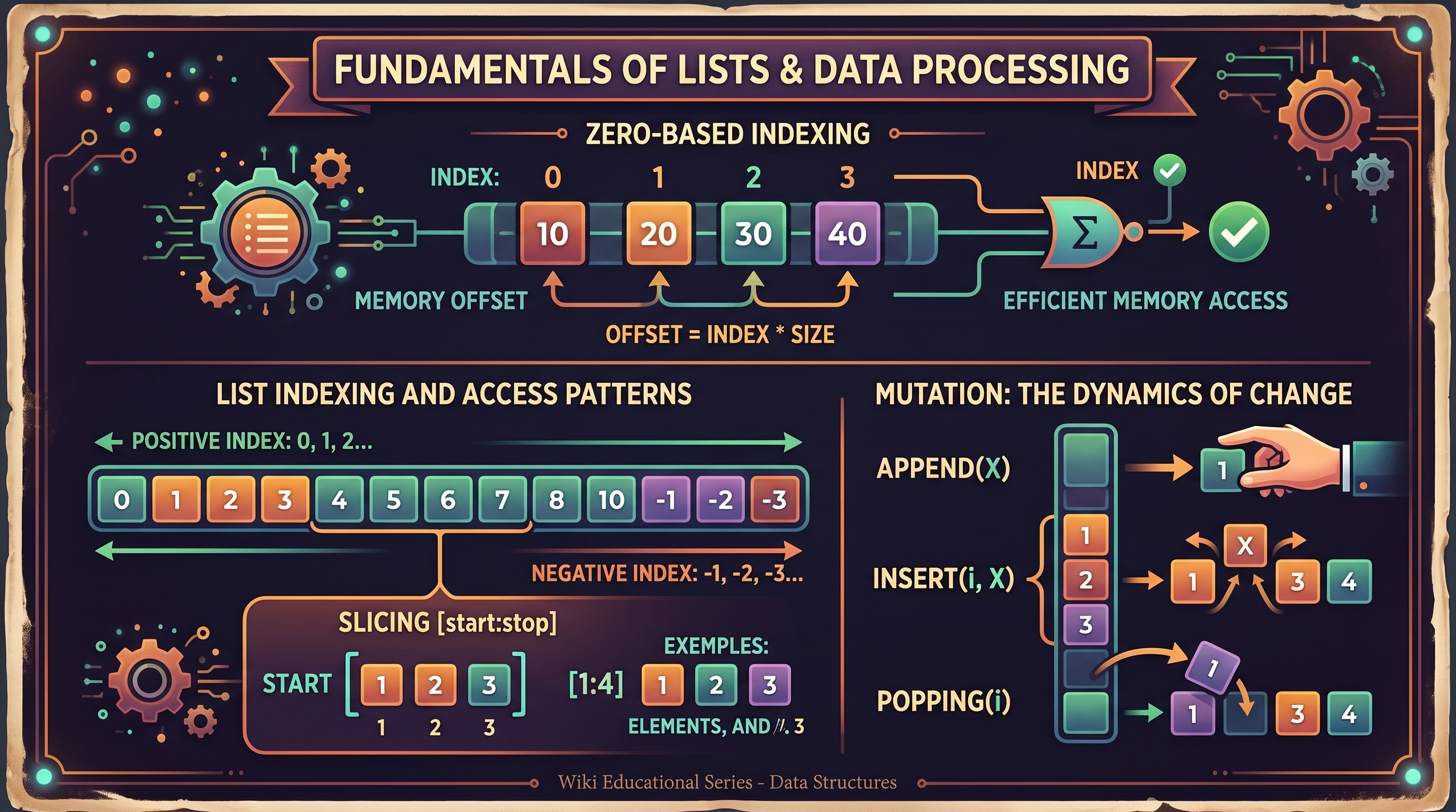
To the uninitiated, starting a count at zero seems counter-intuitive. However, in computer science, Zero-based Indexing is not an arbitrary choice; it is a mathematical necessity derived from how memory is addressed.
Definition: Zero-based Indexing A way of numbering the items in a list where the first item is assigned the index 0, the second item index 1, and so on. For a list of length $n$, the valid indices range from $0$ to $n-1$.
The Memory Offset Derivation
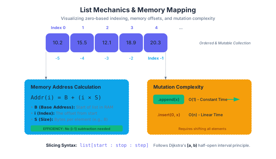
Consider a list stored in a computer's RAM. The list has a Base Address ($B$), which is the memory location of the very first element. Each element in the list occupies a fixed amount of space, let's call it the Size ($S$).
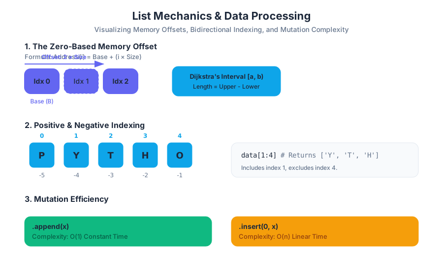
To find the memory address of the $i$-th element, the computer uses the following formula: $$\text{Address}(i) = B + (i \times S)$$
If we used 1-based indexing (where the first element is index 1), the formula would become: $$\text{Address}(i) = B + ((i - 1) \times S)$$
By starting at 0, we eliminate the subtraction operation $(i - 1)$ for every single memory access. In high-performance systems processing billions of data points, saving one subtraction per access results in significant computational efficiency.
Dijkstra’s Argument for $[a, b)$
The legendary computer scientist Edsger W. Dijkstra argued that the most elegant way to represent a range of natural numbers is using a "half-open interval" $[a, b)$, where the lower bound is included and the upper bound is excluded.
- The number of elements in the range is simply $b - a$.
- If we start at 0 and want $n$ elements, the range is $[0, n)$.
- This prevents "off-by-one" errors that frequently plague 1-based systems.
List Indexing and Access Patterns
Accessing an element in a list is an $O(1)$ operation, meaning it takes the same amount of time regardless of whether the list has ten items or ten million. This is because the memory address calculation described above is instantaneous.
Positive and Negative Indexing
Python and several other modern languages support Negative Indexing, which allows developers to reference elements relative to the end of the list.
| Index Type | Formula / Logic | Use Case |
|---|---|---|
| Positive | list[i] |
Accessing known positions from the start. |
| Negative | list[-i] maps to list[len(list) - i] |
Accessing the "last" or "second to last" items without knowing the total length. |
| Slicing | list[start:stop:step] |
Extracting sub-sections of data for batch processing. |
Slicing Mechanics
Slicing creates a new list containing a subset of the original. The syntax list[start:stop] includes the start index but excludes the stop index (following Dijkstra's $[a, b)$ principle).
# Advanced List Access and Slicing in Python
data_stream = [10.2, 15.5, 12.1, 18.9, 20.3, 14.7, 11.8]

# Accessing the tail of the data
last_three = data_stream[-3:]  # [20.3, 14.7, 11.8]

# Strided sampling (every 2nd element)
sampled_data = data_stream[::2] # [10.2, 12.1, 20.3, 11.8]

# Reversing a list via slicing
reversed_stream = data_stream[::-1]

print(f"Original: {data_stream}")
print(f"Sampled: {sampled_data}")
Mutation: The Dynamics of Change
Unlike strings (which are immutable), lists are mutable. This means we can modify the contents of a list without creating a whole new copy in memory. This is critical for "In-place" algorithms and memory efficiency.
Primary Mutation Methods
There are three main ways to mutate a list's structure:
- Append: Adding an element to the end.
- Insert: Adding an element at a specific index, shifting all subsequent elements to the right.
- Removal/Pop: Deleting an element by value or position.
| Method | Syntax | Time Complexity | Description |
|---|---|---|---|
.append(x) |
L.append(5) |
$O(1)$* | Adds x to the end. Highly efficient. |
.insert(i, x) |
L.insert(0, "A") |
$O(n)$ | Adds x at index i. Requires shifting all items after i. |
.extend(iterable) |
L.extend([1, 2]) |
$O(k)$ | Appends all elements from another collection. |
.pop(i) |
L.pop(0) |
$O(n)$ | Removes and returns item at index i. |
L[i] = x |
L[2] = 99 |
$O(1)$ | Direct replacement of an element at a known index. |
The Cost of Insertion While
.append()is usually "free" (constant time),.insert(0, x)is expensive. To put something at the beginning of a list, the computer must move every other item one slot to the right to make room. In a list of 1 million items, an insertion at the start requires 1 million move operations.
Low-Level Representation
In languages like C, a list (array) is a fixed-size block of memory. To "mutate" its size, we must manually allocate a new, larger block and copy the data. Python automates this using a Dynamic Array strategy: it allocates more space than it currently needs (over-allocation). When the "extra" space runs out, it performs a "Resize" operation.
// A low-level look at how indexing works via pointer arithmetic
#include <stdio.h>

int main() {
    int scores[5] = {88, 92, 79, 85, 90};

    // Standard access
    printf("Index 2: %d\n", scores[2]);

    // Pointer arithmetic (The "Under the Hood" reality)
    // *(base_address + offset)
    int *base_ptr = scores;
    printf("Memory Address Access: %d\n", *(base_ptr + 2));

    return 0;
}
Iteration and the Accumulator Pattern
Data processing is rarely about a single element; it is about transforming the entire collection. The most common pattern for this is the Accumulator Pattern.
The Pattern Structure
- Initialize an accumulator variable (e.g.,
total = 0orresults = []). - Iterate through the list using a loop.
- Update the accumulator inside the loop based on some logic.
- Return/Use the final accumulated value.
Worked Example: Filtering and Transforming
Suppose we have a list of sensor readings in Celsius, and we need to filter out errors (readings below -50) and convert the rest to Fahrenheit.
# The Accumulator Pattern in Action
raw_readings = [22.5, -999, 23.1, 19.8, -999, 25.0]
valid_fahrenheit = [] # 1. Initialize

for temp in raw_readings: # 2. Iterate
    if temp > -50:        # Logic: Filter errors
        f = (temp * 9/5) + 32
        valid_fahrenheit.append(f) # 3. Update

print(valid_fahrenheit) # 4. Use result
Strings vs. Lists: The Immutability Divide
While strings and lists both behave like sequences (you can index them, slice them, and loop over them), they differ in one fundamental way: Immutability.
| Feature | Lists | Strings |
|---|---|---|
| Type | Mutable | Immutable |
| Modification | L[0] = 'z' (Allowed) |
S[0] = 'z' (TypeError) |
| Memory | Modified in place | New string created for every change |
| Common Use | Collections of heterogeneous data | Textual data |
String Manipulation via Lists
Because strings are immutable, performing many small changes (like building a sentence word by word) is inefficient. Every time you add a character, a new string is created. The "Pro" way to handle this is to collect characters in a List and then use the .join() method.
# Real-world usage: Processing a list of files in a directory
# We use a shell loop to 'accumulate' filenames into a processing pipeline

files=$(ls *.txt)

for file in $files; do
    echo "Processing $file..."
    # Imagine a complex transformation here
    cat "$file" | tr '[:lower:]' '[:upper:]' > "PROCESSED_$file"
done

echo "Batch processing complete."
Common Pitfalls in List Processing
1. The "Mutation During Iteration" Trap
One of the most common logic errors occurs when a developer tries to remove items from a list while looping through it.
The Bug: When you remove the item at index
i, all subsequent items shift to indexi-1. The loop then moves to indexi+1, effectively skipping the item that just moved into indexi.
Solution: Iterate over a copy of the list (for item in my_list[:]) or use a list comprehension to create a new, filtered list.
2. Shallow vs. Deep Copies
When you write list_b = list_a, you are not creating a new list. You are creating a new "reference" to the same list in memory. Changing list_b will change list_a. To create a truly independent copy, use list_b = list_a.copy().
3. Off-by-One Errors
Because lists are zero-indexed, the last element is at len(list) - 1. Attempting to access list[len(list)] will trigger an IndexError. This is the most frequent runtime error for junior engineers.
Advanced Data Modeling: Nested Lists
Lists can contain other lists, creating multi-dimensional structures like grids, matrices, or tables.
| Row | Col 0 | Col 1 | Col 2 |
|---|---|---|---|
| 0 | Matrix[0][0] | Matrix[0][1] | Matrix[0][2] |
| 1 | Matrix[1][0] | Matrix[1][1] | Matrix[1][2] |
To access an element in a 2D list, you use two indices: matrix[row][column]. This is the basis for image processing (where an image is a 2D list of pixels) and game boards (like Chess or Tic-Tac-Toe).
Source Materials
Study Computing on Lykke
This course page is free to open: signed out, you can read its first two sections, and signing in, on any plan, opens the rest. The free Lykke Chrome extension syncs your own Canvas courses, so ChatGPT, Claude and Muse can answer from your classes and deadlines. It only reads Canvas.
Add the free extensionSign in to open every section