From the free course Computing on Lykke
Functions and Modularity
Key concepts: Function definitions · Parameters · Return statements · Modularity
Organizing code into reusable, independent modules called functions.
Functions and Modularity
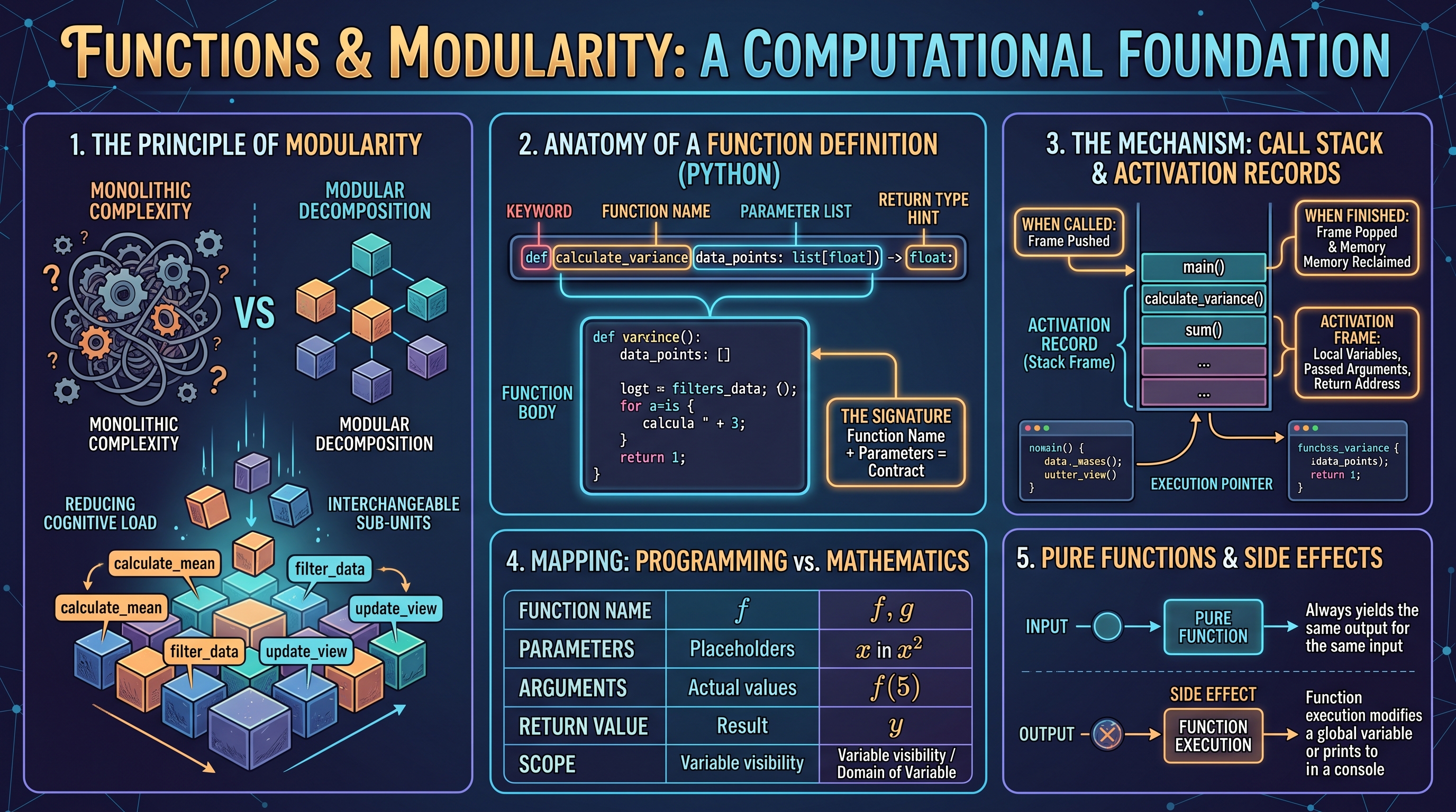
In the realm of software engineering, complexity is the primary antagonist. As a system grows, the cognitive load required to understand its state transitions and logic flow increases exponentially. To combat this, we employ Modularity: the architectural strategy of decomposing a monolithic problem into discrete, independent, and interchangeable sub-units. At the heart of modularity lies the Function.
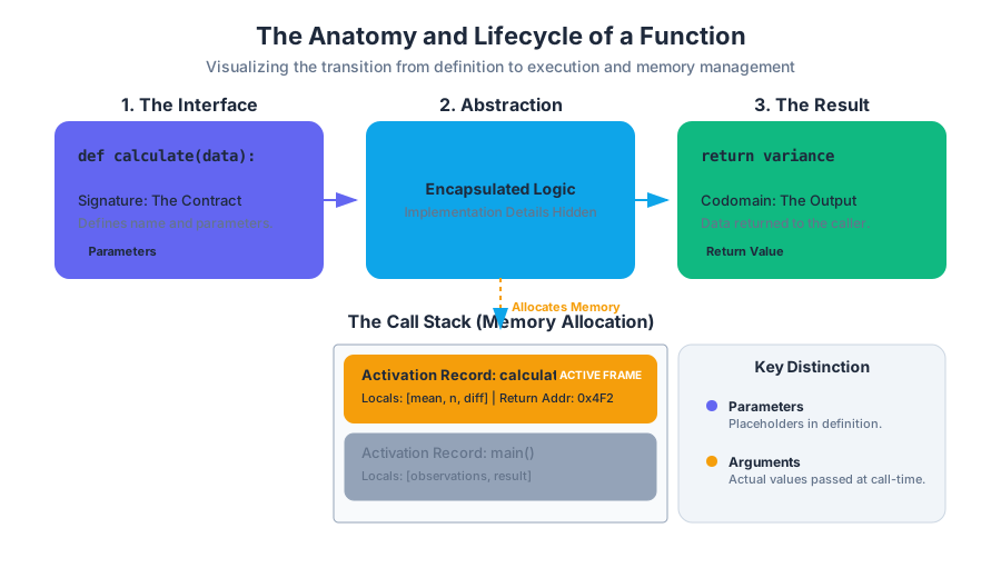
A function is not merely a "block of code"; it is a formal abstraction. It represents a mapping from a set of inputs (the domain) to a set of outputs (the codomain), encapsulated in a way that hides implementation details from the caller. This principle, known as Abstraction, allows us to build "black boxes" where we care about what the code does, rather than how it does it.
The Anatomy of a Function Definition
A Function Definition is the blueprint for a computational task. In Python, this is initiated with the def keyword, followed by the function name, a parameter list, and a colon. This header defines the function's Signature—the contract it makes with the rest of the program.
The body of the function is an indented block of code. When a function is "called" or "invoked," the program's execution pointer jumps to this block, executes the logic, and then returns to the point of origin. This mechanism is managed by the Call Stack, a data structure that tracks active subroutines.
Definition: The Activation Record When a function is called, the system creates an Activation Record (or Stack Frame) on the call stack. This record contains the function's local variables, the arguments passed to it, and the return address. When the function finishes, its frame is "popped" off the stack, and its local memory is reclaimed.
Implementation: A Statistical Analysis Module
The following example demonstrates a non-trivial function designed to calculate the variance of a dataset. It showcases local variable encapsulation and algorithmic logic.
def calculate_variance(data_points: list[float]) -> float:
    """
    Calculates the population variance of a numeric dataset.
    Formula: σ² = Σ(x - μ)² / N
    """
    if not data_points:
        raise ValueError("Dataset cannot be empty.")

    # Step 1: Calculate the arithmetic mean (μ)
    n = len(data_points)
    mean = sum(data_points) / n

    # Step 2: Calculate the sum of squared differences from the mean
    squared_diff_sum = 0.0
    for x in data_points:
        diff = x - mean
        squared_diff_sum += diff ** 2

    # Step 3: Compute variance
    variance = squared_diff_sum / n
    return variance

# Execution context
observations = [10.5, 12.2, 9.8, 11.1, 10.9]
result = calculate_variance(observations)
print(f"Population Variance: {result:.4f}")
Formalizing the Mapping: Mathematical Representation
To understand functions at a fundamental level, we must look at them through the lens of discrete mathematics. A function $f$ is a relation that associates each element $x$ of a set $X$ to exactly one element $y$ of a set $Y$.
f: X \to Y
\text{where } x \in X \text{ is the input and } f(x) \in Y \text{ is the output.}
In programming, we extend this definition to include Side Effects—changes to the state of the system (like printing to a console or modifying a global variable) that occur during the function's execution. A Pure Function is one that has no side effects and always produces the same output for the same input, mirroring the mathematical ideal.
| Concept | Programming Definition | Mathematical Analog |
|---|---|---|
| Function Name | The identifier used to invoke the logic. | The symbol $f$ or $g$. |
| Parameters | Placeholders defined in the function header. | Variables in the expression (e.g., $x$ in $x^2$). |
| Arguments | The actual values passed during a call. | The specific value substituted (e.g., $f(5)$). |
| Return Value | The data sent back to the caller. | The result of the evaluation ($y$). |
| Scope | The visibility of variables. | The domain of the variable. |
Parameters and Arguments: The Input Interface
Parameters are the variables listed in the function's definition. They act as local names for the data the function expects. Arguments are the actual data values supplied to the function when it is called.
Parameter Passing Mechanisms
Different programming languages handle the transmission of arguments differently. Python uses a mechanism often called Pass-by-Object-Reference. This means the function receives a reference to the same object in memory, but the "name" in the function is local.
- Positional Arguments: Mapped to parameters based on their order.
- Keyword Arguments: Mapped by name, allowing for out-of-order passing.
- Default Parameters: Parameters that assume a pre-defined value if the caller provides none.
Comparison of Argument Types
| Type | Syntax Example | Use Case |
|---|---|---|
| Positional | power(2, 10) |
Simple, intuitive mappings. |
| Keyword | connect(host="localhost", port=8080) |
Improving readability in complex signatures. |
| Default | def log(msg, level="INFO"): |
Providing sensible defaults while allowing overrides. |
| *Variadic (args) | def sum_all(*nums): |
Functions that accept an arbitrary number of inputs. |
The Danger of Mutable Defaults
A common pitfall for senior and junior engineers alike is using mutable objects (like lists or dictionaries) as default arguments. In Python, default arguments are evaluated only once at the time of function definition, not at each call.
# ANTI-PATTERN: The list is shared across all calls!
def add_to_registry(name, registry=[]):
    registry.append(name)
    return registry

# CORRECT PATTERN: Use None as a sentinel
def add_to_registry_safe(name, registry=None):
    if registry is None:
        registry = []
    registry.append(name)
    return registry
Return Statements: The Output Pipeline
The return statement serves two purposes: it terminates the function's execution and optionally passes a value back to the calling environment. If a function reaches the end of its block without a return statement, it implicitly returns None.
Multiple Return Points
Functions can have multiple return statements, often used in "guard clauses" to handle edge cases early. This reduces the nesting level of the code (the "Arrow Anti-pattern").
Structural Comparison: Low-Level vs. High-Level Returns
To see how functions handle returns at a lower level, consider how a systems language like Rust manages ownership and return values compared to Python's reference-based approach.
// Rust implementation showing explicit return types and ownership
fn find_max(numbers: &[i32]) -> Option<i32> {
    if numbers.is_empty() {
        return None; // Early return for edge case
    }

    let mut max_val = numbers[0];
    for &val in numbers.iter() {
        if val > max_val {
            max_val = val;
        }
    }
    Some(max_val) // Final expression is returned implicitly in Rust
}

fn main() {
    let data = vec![1, 5, 3, 9, 2];
    match find_max(&data) {
        Some(max) => println!("The maximum is {}", max),
        None => println!("The list was empty"),
    }
}
Scope and the LEGB Rule
Scope defines the region of a program where a particular variable name is accessible. Understanding scope is critical for modularity because it prevents "Namespace Pollution"—where different parts of a program accidentally overwrite each other's data.
Python follows the LEGB Rule for variable resolution:
- L (Local): Names assigned within a function and not declared global.
- E (Enclosing): Names in the local scope of any enclosing functions (relevant in nested functions).
- G (Global): Names assigned at the top-level of a module or declared global.
- B (Built-in): Names pre-installed in the Python interpreter (e.g.,
len,range).
The Principle of Least Privilege A variable should only be visible to the parts of the program that absolutely require it. Use local variables by default and avoid global variables, which create hidden dependencies and make debugging difficult.
Modularity: Designing for Reusability
Modularity is the application of functions to organize logic. A modular program is composed of small, focused functions that do one thing well (Single Responsibility Principle).
Benefits of Modularity
- Reusability: A well-written function can be used in multiple parts of a project or even in different projects.
- Maintainability: If a bug is found in a calculation, you only need to fix it in one function definition rather than in twenty different places.
- Testability: Small functions can be tested in isolation using Unit Tests.
Modularity in Practice: The Pipeline Pattern
In real-world systems, modularity often takes the form of a pipeline, where data flows through a series of discrete transformations.
# A modular pipeline in a Unix-like shell
# Each command is a 'function' that performs one task
cat access.log | grep "404" | awk '{print $7}' | sort | uniq -c | sort -nr
In the example above, each command (grep, awk, sort) is a modular unit. They are "composed" using the pipe operator (|), demonstrating how simple functions can be combined to solve complex data processing problems.
Advanced Modularity: Higher-Order Functions
A Higher-Order Function is a function that either takes another function as an argument or returns a function as its result. This is a cornerstone of functional programming and allows for extreme modularity.
Common examples include map, filter, and reduce. These allow us to abstract the logic of iteration away from the logic of the operation.
| Method | Purpose | Input | Output |
|---|---|---|---|
| Map | Applies a function to every item in a list. | Function + List | New List |
| Filter | Keeps only items that satisfy a condition. | Predicate Function + List | Filtered List |
| Reduce | Combines all items into a single value. | Binary Function + List | Single Value |
Example: Functional Composition
def apply_operation(data, func):
    """A higher-order function that applies 'func' to 'data'."""
    return [func(x) for x in data]

def square(n): return n * n
def cube(n): return n * n * n

nums = [1, 2, 3, 4]
print(apply_operation(nums, square)) # [1, 4, 9, 16]
print(apply_operation(nums, cube))   # [1, 8, 27, 64]
Common Pitfalls and Best Practices
- Side Effects: Avoid modifying global variables inside a function. If a function must change state, return the new state.
- Long Parameter Lists: If a function requires more than 4 or 5 arguments, it likely has too many responsibilities. Consider grouping arguments into a dictionary or an object.
- Deep Nesting: Use early returns to keep the "happy path" of the function at the lowest indentation level.
- Documentation: Always use docstrings to explain the function's purpose, parameters, and return values.
Summary of Modularity Metrics
To evaluate the quality of modular code, engineers often look at two metrics: Cohesion and Coupling.
| Metric | Goal | Description |
|---|---|---|
| Cohesion | High | How closely related the logic inside a single module is. A high-cohesion function does exactly one thing. |
| Coupling | Low | How much one module depends on another. Low coupling means you can change one function without breaking others. |
By maximizing cohesion and minimizing coupling, we create robust architectures that can withstand the evolving requirements of complex software systems.
Source Materials
Study Computing on Lykke
This course page is free to open: signed out, you can read its first two sections, and signing in, on any plan, opens the rest. The free Lykke Chrome extension syncs your own Canvas courses, so ChatGPT, Claude and Muse can answer from your classes and deadlines. It only reads Canvas.
Add the free extensionSign in to open every section