From the free course Statistics and Probability on Lykke
Two-Sample Inference
Key concepts: Difference of Means · Difference of Proportions · Pooled Proportions · Independent Samples · Matched Pairs
Comparing two different populations or treatment groups using means and proportions.
Two-Sample Inference
In the realm of statistical analysis, moving from one-sample inference to Two-Sample Inference represents a shift from simple estimation to comparative science. While one-sample tests ask, "Is the population mean equal to a specific value?", two-sample tests ask, "Is there a fundamental difference between these two populations?" This is the bedrock of the scientific method, enabling us to evaluate the efficacy of medical treatments, the impact of policy changes, or the performance of competing algorithms.
The Fundamental Logic of Comparison
Two-sample inference is built upon the distribution of the difference between statistics. Whether we are comparing means ($\bar{x}_1 - \bar{x}_2$) or proportions ($\hat{p}_1 - \hat{p}_2$), we are essentially creating a new random variable representing the gap between two groups.
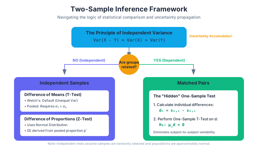
The core challenge lies in the propagation of uncertainty. Because both samples are subject to sampling error, the variance of their difference is the sum of their individual variances (assuming independence). This is derived from the property of variance: $Var(X - Y) = Var(X) + Var(Y)$ for independent variables.
The Principle of Independent Variance: When subtracting two independent random variables, their uncertainties do not cancel out; they accumulate. This is why the standard error of a difference is always larger than the standard error of the individual components.
Independent Samples vs. Matched Pairs
Before selecting a test, the researcher must identify the relationship between the two groups. This distinction dictates the entire mathematical approach.
| Feature | Independent Samples | Matched Pairs (Dependent) |
|---|---|---|
| Data Source | Two distinct, unrelated groups (e.g., Men vs. Women). | The same subjects measured twice, or twins/matched subjects. |
| Sample Sizes | Can be different ($n_1 \neq n_2$). | Must be identical ($n_1 = n_2$). |
| Statistical Goal | Compare the centers of two distributions. | Compare the mean of the differences ($ \mu_d $). |
| Primary Benefit | Simplicity in experimental design. | Controls for subject-to-subject variability; higher power. |
Matched Pairs: The "Hidden" One-Sample Test
In a Matched Pairs design, we do not actually perform a two-sample test. Instead, we calculate the difference $d_i = x_{1,i} - x_{2,i}$ for each pair. We then perform a one-sample t-test on these differences. This effectively eliminates the "noise" caused by individual differences between subjects, focusing solely on the effect of the treatment.
Difference of Means: Independent Samples
When comparing the means of two independent populations, we typically employ the Two-Sample T-Test. This is used when the population standard deviations ($\sigma_1, \sigma_2$) are unknown, which is the case in almost all real-world scenarios.
The Welch’s T-Test vs. Pooled T-Test
There are two primary ways to calculate the t-statistic for independent means:
- Welch’s T-Test (Unpooled): Does not assume equal variances. This is the modern default in software like R and Python (SciPy).
- Pooled T-Test: Assumes $\sigma_1^2 = \sigma_2^2$. While slightly more powerful if the assumption holds, it is risky and often discouraged unless the experimental design guarantees equal variance.
Mathematical Derivation of the T-Statistic
The t-statistic for the difference of means is defined as:
$$t = \frac{(\bar{x}_1 - \bar{x}2) - (\mu_1 - \mu_2)}{SE{\bar{x}_1 - \bar{x}_2}}$$
Where the Standard Error ($SE$) for the unpooled version is:
$$SE = \sqrt{\frac{s_1^2}{n_1} + \frac{s_2^2}{n_2}}$$
Degrees of Freedom (Satterthwaite Approximation)
In a one-sample test, $df = n-1$. In a two-sample test where variances are not assumed equal, the degrees of freedom calculation is notoriously complex. Most students use the "conservative" $df = \min(n_1-1, n_2-1)$, but professional software uses the Satterthwaite-Welch formula:
df \approx \frac{\left( \frac{s_1^2}{n_1} + \frac{s_2^2}{n_2} \right)^2}{\frac{1}{n_1-1}\left(\frac{s_1^2}{n_1}\right)^2 + \frac{1}{n_2-1}\left(\frac{s_2^2}{n_2}\right)^2}
Difference of Proportions
Comparing proportions (e.g., conversion rates in an A/B test) requires a Two-Sample Z-Test. Unlike means, which use the T-distribution to account for estimated standard deviation, proportions use the Normal (Z) distribution because the standard deviation of a proportion is directly tied to the proportion itself ($\sigma_p = \sqrt{p(1-p)/n}$).
The Concept of Pooled Proportions
There is a critical distinction in how we calculate standard error for proportions depending on whether we are building a Confidence Interval or performing a Hypothesis Test.
- Confidence Intervals: We use the individual sample proportions ($\hat{p}_1$ and $\hat{p}_2$) because we are estimating the actual difference.
- Hypothesis Testing: Under the null hypothesis ($H_0: p_1 = p_2$), we assume both samples come from a population with the same proportion. Therefore, we "pool" the data to get the best possible estimate of this common proportion ($p_c$).
Pooled Proportion Formula: $$\hat{p}_c = \frac{X_1 + X_2}{n_1 + n_2}$$ Where $X$ is the number of successes.
Standard Error Comparison
| Context | Standard Error Formula |
|---|---|
| Confidence Interval | $SE = \sqrt{\frac{\hat{p}_1(1-\hat{p}_1)}{n_1} + \frac{\hat{p}_2(1-\hat{p}_2)}{n_2}}$ |
| Hypothesis Test | $SE_{pooled} = \sqrt{\hat{p}_c(1-\hat{p}_c) \left( \frac{1}{n_1} + \frac{1}{n_2} \right)}$ |
Conditions for Valid Inference
For the results of these tests to be valid, several assumptions must be met. Failure to verify these can lead to Type I errors (false positives) or Type II errors (false negatives).
- Independence:
- Within groups: Observations in each sample must be independent (usually satisfied by random sampling or the 10% rule).
- Between groups: The two samples must be independent of each other (unless using a Matched Pairs design).
- Normality / Large Counts:
- For Means: Each population should be Normal, or sample sizes should be large enough ($n > 30$) for the Central Limit Theorem to apply.
- For Proportions: The "Success/Failure" condition must be met for both groups: $np \geq 10$ and $n(1-p) \geq 10$.
- Randomization: Data must come from a random sample or a randomized experiment to generalize results.
Common Pitfalls and Misconceptions
1. Confusing Independent Samples with Matched Pairs
This is the most common error in undergraduate statistics. If you measure the weight of 50 people before a diet and the same 50 people after, you have one sample of 50 differences, not two independent samples of 50. Using an independent t-test here ignores the correlation between the "before" and "after" measurements, drastically reducing the power of the test.
2. The "Equality of Variance" Trap
Many older textbooks emphasize checking for equal variance using an F-test or Levene's test before choosing between a Pooled or Welch's t-test. However, modern statistical theory suggests that Welch's T-test is almost always preferable. It performs nearly as well as the pooled test when variances are equal and far outperforms it when they are not.
3. Over-reliance on P-values
A statistically significant difference (small p-value) does not necessarily mean the difference is practically significant. With large enough sample sizes (e.g., $n=1,000,000$), even a trivial difference in means will produce a significant p-value. Always report the Effect Size (like Cohen's d) alongside the p-value.
4. Pooling Proportions for Confidence Intervals
As noted earlier, you should only pool proportions for hypothesis tests. For confidence intervals, pooling is mathematically inconsistent because the interval is meant to capture the uncertainty of the actual proportions, not a hypothetical shared proportion.
Summary of Inference Procedures
| Scenario | Parameter | Test Statistic | Standard Error |
|---|---|---|---|
| Means (Independent) | $\mu_1 - \mu_2$ | T-score | $\sqrt{\frac{s_1^2}{n_1} + \frac{s_2^2}{n_2}}$ |
| Means (Matched Pairs) | $\mu_d$ | T-score | $\frac{s_d}{\sqrt{n}}$ |
| Proportions (CI) | $p_1 - p_2$ | Z-score | $\sqrt{\frac{\hat{p}_1(1-\hat{p}_1)}{n_1} + \frac{\hat{p}_2(1-\hat{p}_2)}{n_2}}$ |
| Proportions (Test) | $p_1 - p_2$ | Z-score | $\sqrt{\hat{p}_c(1-\hat{p}_c) (\frac{1}{n_1} + \frac{1}{n_2})}$ |
Source Materials
Study Statistics and Probability on Lykke
This course page is free to open: signed out, you can read its first two sections, and signing in, on any plan, opens the rest. The free Lykke Chrome extension syncs your own Canvas courses, so ChatGPT, Claude and Muse can answer from your classes and deadlines. It only reads Canvas.
Add the free extensionSign in to open every sectionAll sections of Statistics and Probability · Browse more course pages