From the free course Statistics and Probability on Lykke
Sampling Distributions and the CLT
Key concepts: Parameters vs. Statistics · Sampling Distribution of a Proportion · Sampling Distribution of a Mean · Central Limit Theorem (CLT) · Unbiased Estimators
Understanding how sample statistics vary and the power of the Central Limit Theorem.
Sampling Distributions and the CLT
In the realm of statistical inference, we are often tasked with a seemingly impossible challenge: making definitive statements about a vast, unreachable population using only a tiny, finite sliver of data. This bridge between the sample and the population is built upon the theory of Sampling Distributions.
If descriptive statistics is the art of summarizing what we see, then sampling distributions are the science of quantifying the uncertainty in what we don't see. They represent a "meta-level" of probability—instead of asking about the probability of a single individual having a certain trait, we ask about the probability of an entire sample's average falling within a specific range.
Parameters vs. Statistics
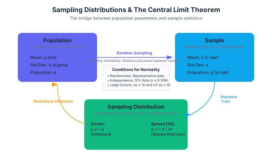
Before we can model the behavior of samples, we must establish a rigorous vocabulary to distinguish between the "truth" of the population and the "estimate" provided by our data. This is the distinction between parameters and statistics.
Definition: A Parameter is a fixed (usually unknown) numerical value that describes an entire population. A Statistic is a numerical value calculated from a sample, which varies from sample to sample.
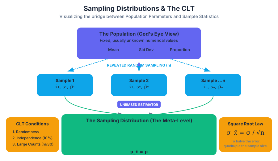
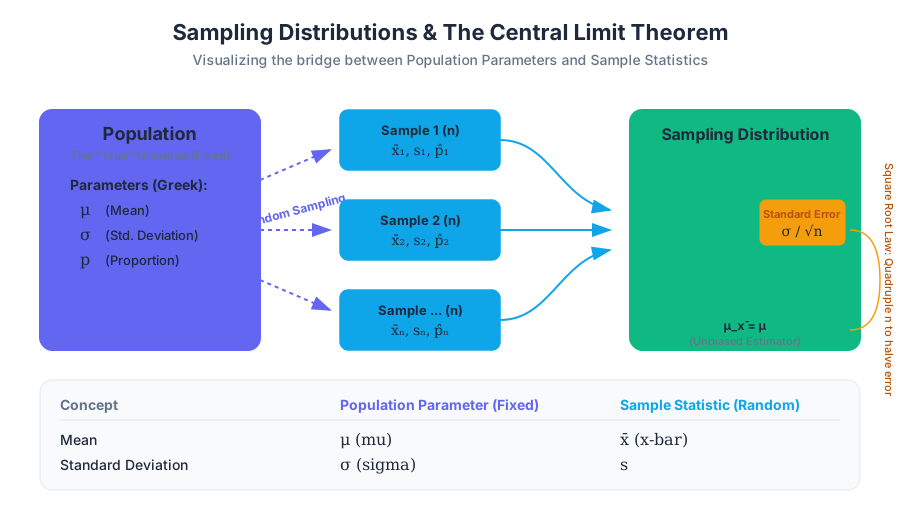
We use specific notation to keep these concepts distinct. In the professor’s shorthand: Greek letters usually denote the "God’s eye view" (parameters), while Latin letters or "hats" denote the "Researcher’s view" (statistics).
| Concept | Population Parameter (Fixed) | Sample Statistic (Random Variable) |
|---|---|---|
| Mean | $\mu$ (mu) | $\bar{x}$ (x-bar) |
| Standard Deviation | $\sigma$ (sigma) | $s$ |
| Proportion | $p$ | $\hat{p}$ (p-hat) |
| Variance | $\sigma^2$ | $s^2$ |
| Correlation | $\rho$ (rho) | $r$ |
The Nature of Sampling Variability
If you take a random sample of 100 students and find an average height of 170cm, and I take a different random sample of 100 students and find 172cm, neither of us is "wrong." This fluctuation is called sampling variability. The sampling distribution is the probability distribution of all possible values of a statistic if we were to repeat the sampling process an infinite number of times.
Unbiased Estimators
A central goal in statistics is to find a sample statistic that serves as a "good" guess for the population parameter. We define "goodness" primarily through the lens of bias and variability.
Accuracy: The Unbiased Property
A statistic is an unbiased estimator of a population parameter if the mean of its sampling distribution is equal to the true value of the parameter being estimated. Mathematically, $\hat{\theta}$ is unbiased for $\theta$ if: $$E[\hat{\theta}] = \theta$$
Precision: Minimum Variance
Even if an estimator is unbiased, it might be "noisy" (high variance). We prefer estimators that are both unbiased and have the smallest possible standard deviation. This is why we use $(n-1)$ in the denominator of the sample variance $s^2$; using $n$ would consistently underestimate the population variance $\sigma^2$, making it a biased estimator.
Sampling Distribution of a Proportion
When dealing with categorical data (e.g., "Yes/No" or "Success/Failure"), we are interested in the proportion $p$ of the population that possesses a certain characteristic. The sample proportion $\hat{p}$ is calculated as $X/n$, where $X$ is the count of successes.
The Mean and Standard Deviation
The sampling distribution of $\hat{p}$ has the following properties:
- Center: $\mu_{\hat{p}} = p$ (The sample proportion is an unbiased estimator).
- Spread: $\sigma_{\hat{p}} = \sqrt{\frac{p(1-p)}{n}}$ (This is often called the Standard Error of the proportion).
Conditions for Normality
We cannot always assume the sampling distribution of $\hat{p}$ is Normal. For the distribution to be approximately Normal, three conditions must be met:
| Condition | Requirement | Purpose |
|---|---|---|
| Randomness | Data must come from a well-designed random sample or randomized experiment. | Ensures the sample is representative and avoids bias. |
| Independence (10% Rule) | When sampling without replacement, $n \le 0.10N$. | Ensures that the probability of success doesn't change significantly between draws. |
| Large Counts | $np \ge 10$ and $n(1-p) \ge 10$. | Ensures the distribution has enough "room" to be symmetric and not "bunched" against 0 or 1. |
Worked Example: Political Polling
Imagine a city where 60% ($p = 0.60$) of voters support a new tax. You survey 400 voters.
- $\mu_{\hat{p}} = 0.60$
- $\sigma_{\hat{p}} = \sqrt{\frac{0.6 \times 0.4}{400}} = \sqrt{0.0006} \approx 0.0245$
- Large Counts check: $400(0.6) = 240$ and $400(0.4) = 160$. Both are $\ge 10$.
- Conclusion: The distribution of your sample proportion is $N(0.60, 0.0245)$.
Sampling Distribution of a Mean
When dealing with quantitative data, we focus on the sample mean $\bar{x}$. This is perhaps the most important concept in all of statistics because it allows us to quantify the precision of scientific measurements.
The Mean and Standard Deviation
- Center: $\mu_{\bar{x}} = \mu$ (The sample mean is an unbiased estimator of the population mean).
- Spread: $\sigma_{\bar{x}} = \frac{\sigma}{\sqrt{n}}$
Key Insight: Notice the $\sqrt{n}$ in the denominator. This is the Square Root Law. To cut your uncertainty (standard error) in half, you must quadruple your sample size. This is why large-scale clinical trials are so expensive; the "returns" on sample size diminish as $n$ grows.
Derivation of the Variance of the Mean
Why is the standard deviation divided by $\sqrt{n}$? We can derive this using the properties of variance for independent random variables $X_1, X_2, ..., X_n$:
\begin{aligned}
Var(\bar{X}) &= Var\left(\frac{\sum X_i}{n}\right) \\
&= \frac{1}{n^2} Var\left(\sum X_i\right) \\
&= \frac{1}{n^2} \sum Var(X_i) \quad \text{(assuming independence)} \\
&= \frac{1}{n^2} (n\sigma^2) = \frac{\sigma^2}{n} \\
\sigma_{\bar{x}} &= \sqrt{\frac{\sigma^2}{n}} = \frac{\sigma}{\sqrt{n}}
\end{aligned}
The Central Limit Theorem (CLT)
The Central Limit Theorem is often called the "Fundamental Theorem of Statistics." It describes the shape of the sampling distribution of the mean.
The Central Limit Theorem: Regardless of the shape of the underlying population distribution, the sampling distribution of the sample mean $\bar{x}$ becomes approximately Normal as the sample size $n$ increases.
Why is this "Magic"?
Most things in the real world are not Normally distributed. Income is skewed right; survival times are exponential; dice rolls are uniform. However, the average of these values will always trend toward a bell curve. This allows us to use Normal probability calculations (Z-scores) even when we don't know the population's shape.
The "Rule of 30"
How large must $n$ be?
- If the population is already Normal, the sampling distribution is Normal for any sample size $n$.
- If the population is skewed or has outliers, we generally need $n \ge 30$ for the CLT to "kick in" and provide a reasonable Normal approximation.
| Population Shape | Sample Size ($n$) | Sampling Distribution Shape |
|---|---|---|
| Normal | $n=2$ | Perfectly Normal |
| Symmetric/Uniform | $n=10$ | Approximately Normal |
| Heavily Skewed | $n=30$ | Approximately Normal |
| Extreme Outliers | $n=100+$ | Approximately Normal |
Practical Usage: Probability Calculations
Once we know that $\bar{x} \sim N(\mu, \frac{\sigma}{\sqrt{n}})$, we can calculate the probability of obtaining a specific sample mean using Z-scores.
The Z-score for a Sample Mean
The formula for a single individual is $z = \frac{x - \mu}{\sigma}$. The formula for a sample mean is: $$z = \frac{\bar{x} - \mu}{\sigma / \sqrt{n}}$$
Worked Example: Industrial Quality Control
A factory produces bolts with a mean diameter of 10mm and a standard deviation of 0.2mm. A quality control inspector takes a random sample of 25 bolts. What is the probability that the sample mean diameter is greater than 10.05mm?
- Identify Parameters: $\mu = 10$, $\sigma = 0.2$, $n = 25$.
- Check Conditions: $n=25$ is close to 30; if the population is roughly symmetric, CLT applies.
- Calculate Standard Error: $\sigma_{\bar{x}} = \frac{0.2}{\sqrt{25}} = \frac{0.2}{5} = 0.04$.
- Calculate Z-score: $$z = \frac{10.05 - 10}{0.04} = \frac{0.05}{0.04} = 1.25$$
- Find Probability: Using a standard Normal table, $P(Z > 1.25) \approx 0.1056$. There is a 10.56% chance the inspector finds a sample mean this high purely by random chance.
Comparison of Distributions
It is vital to distinguish between three distinct types of distributions that students often conflate.
| Distribution | What it describes | Mean | Standard Deviation |
|---|---|---|---|
| Population Distribution | Every individual in the entire group. | $\mu$ | $\sigma$ |
| Sample Distribution | The individuals in a single specific sample. | $\bar{x}$ | $s$ |
| Sampling Distribution | The behavior of a statistic over many samples. | $\mu_{\bar{x}} = \mu$ | $\sigma_{\bar{x}} = \sigma / \sqrt{n}$ |
Common Pitfalls and Misconceptions
1. The "Law of Averages" Fallacy
Many people believe that if a sample mean is currently "too high," the next few data points must be "low" to balance it out. This is false. The CLT works through swamping, not compensation. As $n$ increases, the existing "error" is divided by a larger and larger number, making its impact on the average negligible.
2. Confusing $n$ with $N$
The standard error formula $\sigma/\sqrt{n}$ depends on the sample size ($n$), not the population size ($N$). A sample of 1,000 people provides the same level of precision whether the population is 100,000 or 100,000,000 (provided the 10% rule is met).
3. Standard Deviation vs. Standard Error
- Standard Deviation measures the dispersion of individual data points.
- Standard Error measures the dispersion of a sample statistic. As $n$ increases, the standard deviation of the sample ($s$) stays roughly the same (it estimates $\sigma$), but the standard error ($\sigma/\sqrt{n}$) decreases.
4. The Normality Assumption
The CLT says the sampling distribution is Normal, not the population. You can have a perfectly Normal sampling distribution even if your population looks like a "U" shape or a uniform block.
Final Summary for the Practitioner
The power of the Central Limit Theorem lies in its universality. It is the reason we can conduct medical trials, perform exit polls during elections, and maintain quality control in manufacturing. By understanding that the mean of a sample is itself a random variable with a predictable shape, center, and spread, we transform "guessing" into "inference."
When you look at a sample mean, do not see a single point. See a single draw from a beautiful, bell-shaped distribution centered at the truth, with a width determined by the square root of your effort ($n$).
Source Materials
Study Statistics and Probability on Lykke
This course page is free to open: signed out, you can read its first two sections, and signing in, on any plan, opens the rest. The free Lykke Chrome extension syncs your own Canvas courses, so ChatGPT, Claude and Muse can answer from your classes and deadlines. It only reads Canvas.
Add the free extensionSign in to open every sectionAll sections of Statistics and Probability · Browse more course pages