From the free course Statistics and Probability on Lykke
Random Variables and Distributions
Key concepts: Discrete vs. Continuous Random Variables · Expected Value (Mean) · Binomial Distributions · Geometric Distributions · Variance of Random Variables
Studying discrete and continuous random variables and their expected values.
Random Variables and Distributions
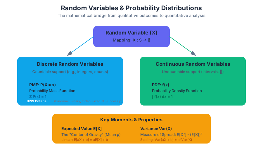
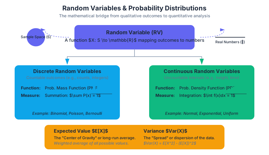
In the rigorous study of probability, a Random Variable (RV) is the formal mechanism that bridges the gap between qualitative outcomes and quantitative analysis. While a sample space might contain outcomes like "Heads" or "Failure," a random variable maps these outcomes to a measurable numerical value, $X: S \to \mathbb{R}$. This mapping allows us to apply the full power of calculus and algebra to uncertain events.
Discrete vs. Continuous Random Variables
The classification of a random variable depends entirely on the nature of its Support—the set of all possible values it can take. Understanding this distinction is critical because the mathematical tools used for each (summation vs. integration) are fundamentally different.
Discrete Random Variables
A Discrete Random Variable has a countable number of possible values. These values are often integers, representing counts (e.g., the number of packets dropped in a network or the number of customers arriving at a bank).
The probability structure of a discrete RV is defined by its Probability Mass Function (PMF), denoted as $P(X = x)$. The PMF must satisfy two primary conditions:
- $0 \le P(X = x) \le 1$ for all $x$.
- $\sum P(X = x) = 1$, where the sum is taken over all possible values of $x$.
Continuous Random Variables
A Continuous Random Variable takes on any value within an interval or collection of intervals. Because there are infinitely many values in any interval, the probability of a continuous RV taking on a specific exact value is zero: $P(X = 1.000...) = 0$.
Instead of a PMF, we use a Probability Density Function (PDF), denoted $f(x)$. Probability is represented by the area under the curve of the PDF over an interval $[a, b]$.
| Feature | Discrete Random Variables | Continuous Random Variables |
|---|---|---|
| Values | Countable (finite or infinite) | Uncountable (intervals) |
| Probability Function | Probability Mass Function (PMF) | Probability Density Function (PDF) |
| $P(X = x)$ | Can be $> 0$ | Always $0$ |
| Total Measure | $\sum P(x) = 1$ | $\int_{-\infty}^{\infty} f(x) dx = 1$ |
| Visualization | Histograms / Bar charts | Smooth density curves |
Expected Value (The Mean of a Distribution)
The Expected Value, denoted $E[X]$ or $\mu$, is the long-run theoretical average of a random variable. It is not necessarily a value the variable will ever actually take; rather, it is the center of gravity of the probability distribution.
Mathematical Definition
For a discrete random variable $X$ with values $x_i$ and probabilities $p_i$, the expected value is the weighted average: $$E[X] = \sum_{i} x_i \cdot P(X = x_i)$$
For a continuous random variable: $$E[X] = \int_{-\infty}^{\infty} x \cdot f(x) dx$$
Linearity of Expectation
One of the most powerful properties in probability is the Linearity of Expectation. For any two random variables $X$ and $Y$ (regardless of whether they are independent), and constants $a$ and $b$: $$E[aX + bY] = aE[X] + bE[Y]$$
Theorem: The Law of the Unconscious Statistician (LOTUS) To find the expected value of a function of a random variable, $g(X)$, you do not need to find the distribution of $g(X)$ first. You can calculate it directly: $E[g(X)] = \sum g(x) P(X=x)$
Variance and Standard Deviation
While the expected value identifies the center, Variance ($Var(X)$ or $\sigma^2$) measures the "spread" or dispersion of the values around that center. It is defined as the expected squared deviation from the mean:
$$Var(X) = E[(X - \mu)^2]$$
The Computational Formula
In practice, we rarely use the definition to calculate variance. Instead, we use the computationally efficient identity: $$Var(X) = E[X^2] - (E[X])^2$$
Properties of Variance
Unlike expectation, variance is not linear. For a constant $a$ and $b$:
- $Var(aX + b) = a^2 Var(X)$ (Adding a constant doesn't change spread; scaling does so quadratically).
- If $X$ and $Y$ are independent: $Var(X + Y) = Var(X) + Var(Y)$.
Binomial Distributions
The Binomial Distribution is the discrete probability distribution of the number of successes in a sequence of $n$ independent experiments.
The BINS Criteria
To use the Binomial model, four conditions must be met:
- Binary: Outcomes must be classified as "Success" or "Failure."
- Independent: The outcome of one trial must not affect the next.
- Number: There is a fixed number of trials ($n$).
- Success: The probability of success ($p$) is constant for each trial.
The Probability Mass Function
The probability of getting exactly $k$ successes in $n$ trials is: $$P(X = k) = \binom{n}{k} p^k (1-p)^{n-k}$$ Where $\binom{n}{k} = \frac{n!}{k!(n-k)!}$ is the binomial coefficient, representing the number of ways to arrange $k$ successes.
Parameters and Moments
- Mean: $E[X] = np$
- Variance: $Var(X) = np(1-p)$
\text{Derivation of Binomial Mean } E[X]:
\text{Let } X = X_1 + X_2 + ... + X_n \text{ where } X_i \text{ is a Bernoulli trial.}
E[X_i] = (1 \cdot p) + (0 \cdot (1-p)) = p
\text{By Linearity of Expectation:}
E[X] = E[X_1] + E[X_2] + ... + E[X_n]
E[X] = p + p + ... + p = np
Geometric Distributions
The Geometric Distribution models the number of trials required to achieve the first success. Unlike the Binomial distribution, the number of trials is not fixed; it is the random variable itself.
Characteristics
- The trials are independent Bernoulli trials.
- The variable $X$ is the trial number of the first success.
- The support is $x \in {1, 2, 3, ...}$.
The Probability Mass Function
To have the first success on trial $k$, you must have $k-1$ failures followed by exactly one success: $$P(X = k) = (1-p)^{k-1} p$$
The Memoryless Property
The Geometric distribution is unique among discrete distributions for being memoryless. This means that the probability of needing $s$ additional trials, given that $t$ trials have already failed, is the same as the initial probability of needing $s$ trials. $$P(X > t + s | X > t) = P(X > s)$$
| Distribution | Random Variable ($X$) | Parameters | Mean ($E[X]$) | Variance ($Var(X)$) |
|---|---|---|---|---|
| Binomial | # of successes in $n$ trials | $n, p$ | $np$ | $np(1-p)$ |
| Geometric | # of trials until 1st success | $p$ | $1/p$ | $(1-p)/p^2$ |
Transforming and Combining Random Variables
In engineering and data science, we rarely look at a single variable in isolation. We often combine them (e.g., the total weight of 10 components or the difference in latency between two servers).
Linear Transformations
If $Y = aX + b$, then:
- $\mu_Y = a\mu_X + b$
- $\sigma_Y = |a|\sigma_X$
- $\sigma^2_Y = a^2\sigma^2_X$
Sums of Independent Random Variables
If $X$ and $Y$ are independent random variables:
- Mean: $\mu_{X+Y} = \mu_X + \mu_Y$
- Variance: $\sigma^2_{X+Y} = \sigma^2_X + \sigma^2_Y$
- Standard Deviation: $\sigma_{X+Y} = \sqrt{\sigma^2_X + \sigma^2_Y}$
Crucial Pitfall: Standard deviations do not add. You must always add variances and then take the square root. This is essentially the Pythagorean Theorem of Statistics.
Common Pitfalls in Distribution Analysis
- Confusing Binomial and Geometric: Always ask: "Is the number of trials fixed?" If yes, it's Binomial. If we are "waiting" for an event, it's Geometric.
- Independence Assumption: Applying $Var(X+Y) = Var(X) + Var(Y)$ to dependent variables. If variables are correlated, you must include the covariance term: $Var(X+Y) = Var(X) + Var(Y) + 2Cov(X,Y)$.
- Continuous Probability Paradox: Forgetting that $P(X=x) = 0$ for continuous variables. This often leads to confusion when calculating the CDF vs. the PDF.
- Scaling Variance: Forgetting to square the constant when moving it out of the variance operator ($Var(3X) = 9Var(X)$, not $3Var(X)$).
Summary of Key Formulas
General Random Variables
- Expected Value: $E[X] = \sum x P(x)$
- Variance: $Var(X) = E[X^2] - (E[X])^2$
- Standard Deviation: $\sigma = \sqrt{Var(X)}$
Binomial Distribution ($X \sim B(n, p)$)
- PMF: $P(X=k) = \binom{n}{k} p^k (1-p)^{n-k}$
- Mean: $np$
- Variance: $np(1-p)$
Geometric Distribution ($X \sim G(p)$)
- PMF: $P(X=k) = (1-p)^{k-1} p$
- Mean: $1/p$
- Variance: $(1-p)/p^2$
Source Materials
Study Statistics and Probability on Lykke
This course page is free to open: signed out, you can read its first two sections, and signing in, on any plan, opens the rest. The free Lykke Chrome extension syncs your own Canvas courses, so ChatGPT, Claude and Muse can answer from your classes and deadlines. It only reads Canvas.
Add the free extensionSign in to open every sectionAll sections of Statistics and Probability · Browse more course pages