From the free course Statistics and Probability on Lykke
Displaying and Summarizing Quantitative Data
Key concepts: Histograms and Dot Plots · Mean and Median · Standard Deviation · Interquartile Range (IQR) · Box Plots and Outliers
Methods for representing numerical data graphically and summarizing it using measures of center and spread.
Displaying and Summarizing Quantitative Data
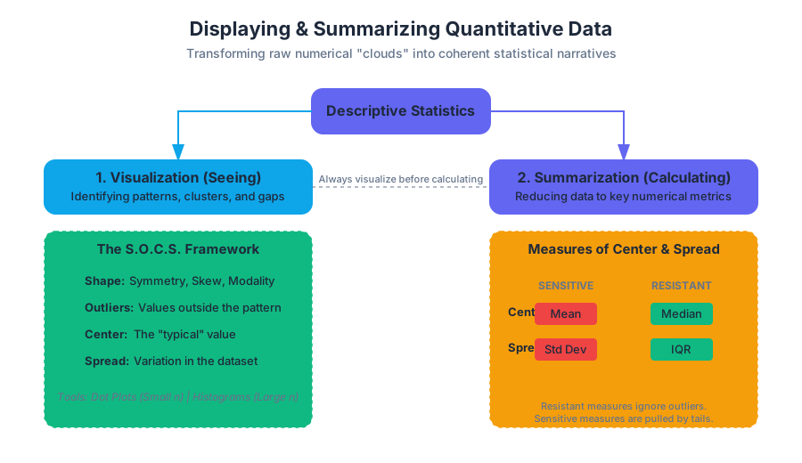
In the realm of statistical analysis, data is generally bifurcated into two categories: categorical (qualitative) and numerical (quantitative). While categorical data deals with labels and attributes, quantitative data represents measurable quantities where arithmetic operations provide meaningful insights. The challenge for the statistician is to transform a raw "cloud" of numbers into a coherent narrative. This process, known as Descriptive Statistics, relies on two primary pillars: Visualization (seeing the data) and Summarization (calculating the data).
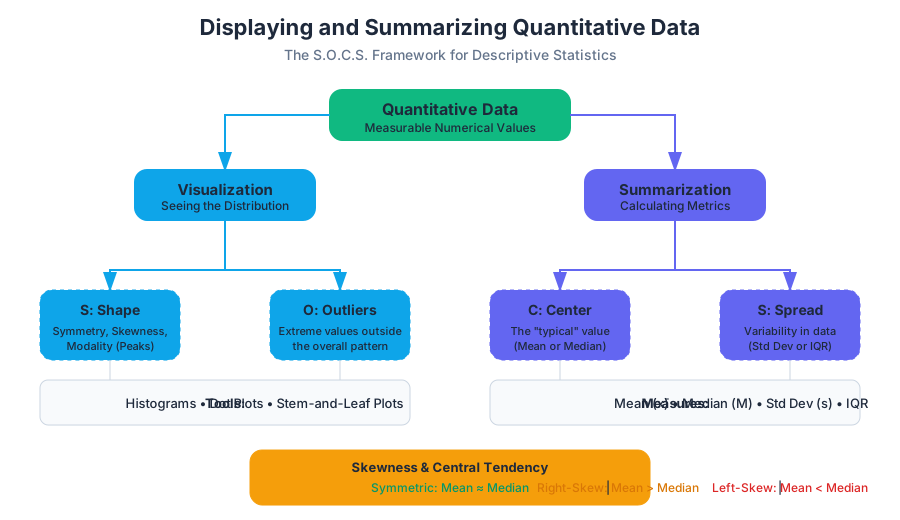
To understand a quantitative distribution, we must examine its S.O.C.S.:
- Shape: Is it symmetric, skewed, unimodal, or bimodal?
- Outliers: Are there individual values that fall outside the overall pattern?
- Center: What is a "typical" value?
- Spread: How much variation exists in the data?
Visualizing Quantitative Distributions
Before calculating a single average, a researcher must look at the data. Graphical displays reveal patterns—clusters, gaps, and skewness—that numerical summaries often hide.
Dot Plots and Stem-and-Leaf Plots
For small datasets, Dot Plots provide the most granular view. Each data point is represented by a dot above a number line. This allows for an immediate assessment of the frequency and the exact location of every value. Similarly, Stem-and-Leaf Plots (or stemplots) preserve the individual data values while grouping them. The "stem" represents the leading digit(s), and the "leaf" represents the final digit.
Histograms
As datasets grow into the thousands or millions, individual dots become illegible. Histograms solve this by grouping adjacent values into bins (or intervals). The height of each bar represents the frequency (count) or relative frequency (percentage) of values falling within that bin.
The Binning Rule: The choice of bin width is critical. Bins that are too wide will "oversmooth" the data, hiding important features like bimodality. Bins that are too narrow will create a "noisy" plot where the overall shape is lost in local fluctuations.
| Feature | Dot Plot | Stem-and-Leaf | Histogram |
|---|---|---|---|
| Data Size | Small ($n < 50$) | Small to Medium | Large ($n > 100$) |
| Granularity | High (shows every point) | High (shows every point) | Low (aggregates into bins) |
| Ease of Construction | Manual/Simple | Manual/Simple | Computational |
| Best Use Case | Initial data inspection | Classroom settings | Professional reporting/Big Data |
Measures of Center: Mean vs. Median
The "center" of a distribution is the value that represents the typical observation. However, "typical" can be defined in multiple ways, leading to the two most common measures: the Arithmetic Mean and the Median.
The Arithmetic Mean ($\bar{x}$)
The mean is the "balance point" of the distribution. Mathematically, it is the sum of all observations divided by the number of observations.
$$\bar{x} = \frac{\sum_{i=1}^{n} x_i}{n}$$
The mean is highly sensitive to outliers. A single extreme value (like a billionaire entering a room of middle-class earners) will pull the mean toward it, often resulting in a value that does not accurately represent the majority of the group.
The Median ($M$)
The median is the "middle" value when the data is arranged in ascending order. If $n$ is odd, the median is the center observation. If $n$ is even, the median is the average of the two center observations.
Unlike the mean, the median is resistant (or robust). It ignores the actual magnitude of extreme values, focusing only on their position.
Shape and Central Tendency
The relationship between the mean and median reveals the skewness of the data:
- Symmetric: Mean $\approx$ Median.
- Right-Skewed (Positive): Mean > Median (the tail pulls the mean to the right).
- Left-Skewed (Negative): Mean < Median (the tail pulls the mean to the left).
Measures of Variability: Standard Deviation and IQR
Knowing the center is insufficient. Two datasets can have the same mean but look entirely different. Spread (or variability) describes how much the data deviates from the center.
Standard Deviation ($s$)
The standard deviation measures the "typical" distance of the observations from the mean. To calculate it, we first find the Variance ($s^2$), which is the average of the squared deviations.
Bessel's Correction: When calculating the sample variance, we divide by $n-1$ rather than $n$. This corrects the bias in the estimation of the population variance, as sample observations tend to be less spread out than the entire population.
\text{Sample Variance: } s^2 = \frac{\sum (x_i - \bar{x})^2}{n - 1}
\text{Standard Deviation: } s = \sqrt{\frac{\sum (x_i - \bar{x})^2}{n - 1}}
The Interquartile Range (IQR)
While the standard deviation is paired with the mean, the IQR is paired with the median. The IQR measures the spread of the middle 50% of the data.
- Q1 (First Quartile): The median of the lower half of the data (25th percentile).
- Q3 (Third Quartile): The median of the upper half of the data (75th percentile).
- IQR = $Q_3 - Q_1$.
Like the median, the IQR is resistant to outliers.
| Metric | Formula/Logic | Sensitivity to Outliers | Best for... |
|---|---|---|---|
| Range | Max - Min | Extremely Sensitive | Quick, rough estimate |
| Standard Deviation | $\sqrt{Var}$ | Sensitive | Symmetric distributions |
| IQR | $Q_3 - Q_1$ | Resistant | Skewed distributions |
| MAD | $\frac{\sum \vert x_i - \bar{x}\vert }{n}$ | Moderate | Intuitive "average error" |
Identifying Outliers: The 1.5xIQR Rule
An outlier is not just a "large number"; it is a point that is mathematically distant from the rest of the data. The most common standard for identifying outliers is the 1.5xIQR Rule, established by John Tukey.
The Algorithm
- Calculate the IQR ($Q_3 - Q_1$).
- Multiply the IQR by 1.5.
- Determine the Lower Bound: $Q_1 - (1.5 \times IQR)$.
- Determine the Upper Bound: $Q_3 + (1.5 \times IQR)$.
- Any data point falling below the Lower Bound or above the Upper Bound is considered a formal outlier.
Why 1.5?
The multiplier 1.5 is a heuristic. In a perfectly Normal (bell-shaped) distribution, the 1.5xIQR rule identifies approximately 0.7% of the data as outliers (points roughly 2.7 standard deviations away from the mean). It provides a balance between being too sensitive (labeling normal variation as outliers) and too restrictive (missing genuine anomalies).
Box and Whisker Plots
The Box Plot is a visual representation of the Five-Number Summary:
- Minimum (non-outlier)
- $Q_1$
- Median
- $Q_3$
- Maximum (non-outlier)
Construction Mechanics
- The Box spans from $Q_1$ to $Q_3$, representing the IQR.
- A Line is drawn inside the box at the Median.
- The Whiskers extend from the box to the smallest and largest values that are not outliers.
- Outliers are typically plotted as individual points (dots or asterisks) beyond the whiskers.
Box plots are exceptionally useful for comparing groups. By placing box plots side-by-side, a researcher can instantly compare the centers (medians), spreads (IQR/Whiskers), and the presence of outliers across different categories.
Linear Transformations and Data Scaling
In many engineering and data science contexts, we must transform data—for example, converting temperatures from Celsius to Fahrenheit or normalizing scores. These transformations have predictable effects on our summary statistics.
Shifting (Addition/Subtraction)
Adding a constant $a$ to every value in a dataset:
- Center: Increases by $a$ (Mean${new}$ = Mean${old} + a$).
- Spread: Remains unchanged (SD and IQR stay the same).
Scaling (Multiplication/Division)
Multiplying every value by a constant $b$:
- Center: Multiplied by $b$.
- Spread: Multiplied by $|b|$.
| Transformation | Mean | Median | Std Dev | IQR | Range |
|---|---|---|---|---|---|
| Add $a$ | $+ a$ | $+ a$ | No Change | No Change | No Change |
| Multiply by $b$ | $\times b$ | $\times b$ | $\times \Vert b\Vert $ | $\times \Vert b\Vert $ | $\times \Vert b\Vert $ |
Common Pitfalls in Summarizing Data
- The "Average" Trap: Reporting only the mean for highly skewed data (like income or house prices). This often misleads the audience by presenting a "typical" value that is much higher than what most people experience.
- Ignoring the Shape: Two distributions can have the same mean and standard deviation but different shapes (e.g., one unimodal and one bimodal). Always visualize before summarizing.
- Standard Deviation on Skewed Data: Using $s$ to describe spread in a heavily skewed distribution is technically possible but often unhelpful, as $s$ is not resistant. The IQR is the preferred metric here.
- Bin Width Bias: In histograms, choosing an arbitrary bin width can hide gaps in the data. If the data represents ages, bins of 10 years might hide a "missing generation" that bins of 1 year would reveal.
- Confusing Sample vs. Population: Forgetting to use $n-1$ for sample standard deviation leads to an underestimation of the true population variability.
Summary of Best Practices
When tasked with displaying and summarizing quantitative data, follow this pipeline:
- Visualize: Create a histogram or dot plot to determine the shape.
- Check for Outliers: Use the 1.5xIQR rule to identify and investigate anomalies. Decide if they are data entry errors or genuine (and interesting) extreme cases.
- Choose Metrics:
- If Symmetric: Use Mean and Standard Deviation.
- If Skewed: Use Median and IQR.
- Compare: If comparing multiple groups, use side-by-side box plots to highlight differences in center and variability.
Source Materials
Study Statistics and Probability on Lykke
This course page is free to open: signed out, you can read its first two sections, and signing in, on any plan, opens the rest. The free Lykke Chrome extension syncs your own Canvas courses, so ChatGPT, Claude and Muse can answer from your classes and deadlines. It only reads Canvas.
Add the free extensionSign in to open every sectionAll sections of Statistics and Probability · Browse more course pages