From the free course Statistics and Probability on Lykke
Estimating with Confidence Intervals
Key concepts: Point Estimates · Margin of Error · Critical Values (z* and t*) · Confidence Level · T-distributions
Constructing intervals to estimate population parameters with a specific level of confidence.
Estimating with Confidence Intervals
In the realm of statistical inference, we are often tasked with a fundamental challenge: how do we describe a vast population using only a tiny, imperfect slice of data? While descriptive statistics allow us to summarize the data we have, Inferential Statistics allows us to make claims about the data we don't have.
The most basic form of inference is the Point Estimate, a single value (like a sample mean $\bar{x}$) used to estimate a population parameter (like the population mean $\mu$). However, point estimates are almost certainly "wrong" in the sense that they rarely equal the exact population parameter. To account for this inherent sampling variability, we use Confidence Intervals (CI). A confidence interval provides a range of plausible values for the parameter, accompanied by a specific level of confidence that the range actually captures the truth.
The Anatomy of a Confidence Interval
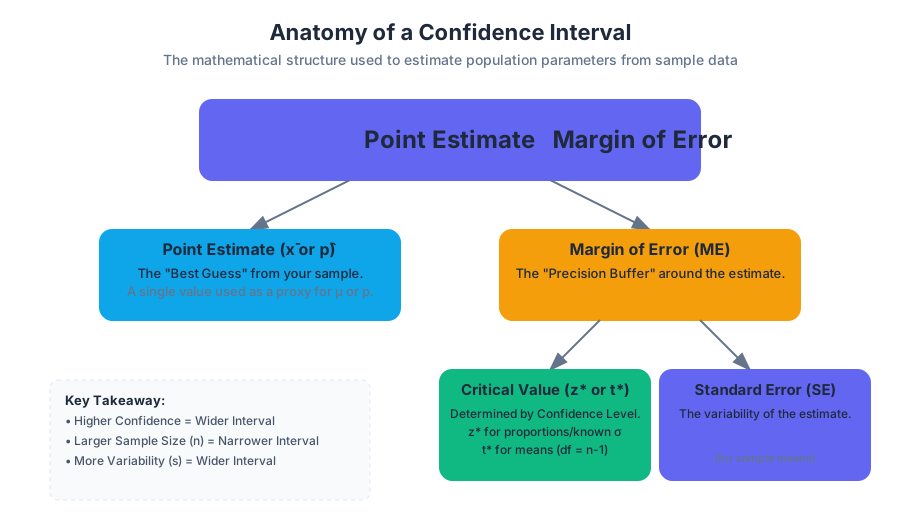
Every confidence interval follows a consistent logical structure. It is built by taking a point estimate and adding or subtracting a Margin of Error (MoE).
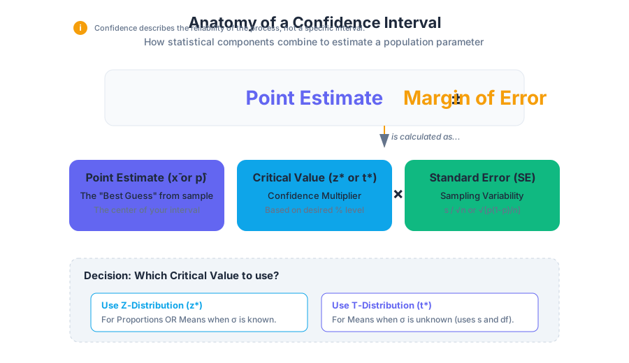
Definition: Confidence Interval A confidence interval is an interval of the form: $$\text{Point Estimate} \pm \text{Margin of Error}$$ Where the Margin of Error is calculated as: $$\text{Margin of Error} = (\text{Critical Value}) \times (\text{Standard Error of the Estimate})$$
The Critical Value ($z^$ or $t^$) is determined by the desired confidence level, while the Standard Error represents the standard deviation of the sampling distribution—essentially, how much we expect the point estimate to fluctuate from sample to sample.
| Component | Symbol | Description |
|---|---|---|
| Point Estimate | $\hat{\theta}$ | The best "single guess" (e.g., $\bar{x}$ or $\hat{p}$) derived from sample data. |
| Confidence Level | $C$ | The success rate of the method (e.g., 95%, 99%). |
| Critical Value | $z^$ or $t^$ | A multiplier that scales the interval based on the confidence level and distribution shape. |
| Standard Error | $SE$ | The estimated standard deviation of the point estimate's sampling distribution. |
| Margin of Error | $ME$ | The maximum expected distance between the point estimate and the true parameter. |
The Philosophy of Confidence Levels
A common misconception is that a "95% confidence interval" means there is a 95% probability that the population parameter lies within that specific interval. In frequentist statistics, the population parameter is a fixed (though unknown) constant. It does not "move." Instead, the interval is what varies from sample to sample.
When we say we are "95% confident," we are describing the reliability of the process. If we were to take 100 different random samples and construct 100 different intervals using the same methodology, approximately 95 of those intervals would successfully capture the true population parameter, and 5 would miss it.
Critical Values: $z^$ vs. $t^$
The choice of the critical value depends on what we know about the population and the type of data we are analyzing.
The Z-Distribution ($z^*$)
We use the Standard Normal Distribution ($z$-scores) when constructing intervals for proportions or when the population standard deviation ($\sigma$) is known (which is rare in practice). The critical value $z^*$ represents the number of standard deviations you must move away from the mean to capture the central $C%$ of the distribution.
| Confidence Level | Alpha ($\alpha$) | Tail Area ($\alpha/2$) | Critical Value ($z^*$) |
|---|---|---|---|
| 90% | 0.10 | 0.05 | 1.645 |
| 95% | 0.05 | 0.025 | 1.960 |
| 99% | 0.01 | 0.005 | 2.576 |
The T-Distribution ($t^*$)
In most real-world scenarios involving means, we do not know the population standard deviation $\sigma$. Instead, we must use the sample standard deviation $s$. Because $s$ is itself an estimate, it introduces extra uncertainty. To compensate, we use the Student’s T-distribution.
The T-distribution is "fatter" in the tails than the Z-distribution. As the sample size $n$ increases, the T-distribution approaches the Normal distribution. The specific shape of the T-distribution is determined by its Degrees of Freedom (df), calculated as $df = n - 1$.
Calculating Intervals for Means
To calculate a confidence interval for a population mean $\mu$ when $\sigma$ is unknown, we follow these steps:
- Verify Conditions: Ensure the sample is random, independent ($n < 10%$ of population), and the population is nearly normal (or $n \ge 30$ per the Central Limit Theorem).
- Calculate Point Estimate: Find the sample mean $\bar{x}$.
- Find Standard Error: $SE_{\bar{x}} = \frac{s}{\sqrt{n}}$.
- Identify Critical Value: Find $t^*$ for $df = n-1$ and the desired confidence level.
- Compute Interval: $\bar{x} \pm t^* \left( \frac{s}{\sqrt{n}} \right)$.
Mathematical Derivation: Sample Size Determination
A common engineering and research question is: "How large must my sample be to ensure my estimate is within a certain margin of error?" We can derive the required sample size $n$ by rearranging the Margin of Error formula.
Derivation for Proportions
For a population proportion $p$, the Margin of Error is: $$ME = z^* \sqrt{\frac{\hat{p}(1-\hat{p})}{n}}$$
To solve for $n$:
- Square both sides: $ME^2 = (z^*)^2 \frac{\hat{p}(1-\hat{p})}{n}$
- Multiply by $n$: $n \cdot ME^2 = (z^*)^2 \hat{p}(1-\hat{p})$
- Divide by $ME^2$: $n = \frac{(z^*)^2 \hat{p}(1-\hat{p})}{ME^2}$
Note: If we don't have a preliminary estimate for $\hat{p}$, we use $\hat{p} = 0.5$ as a "worst-case scenario" because it maximizes the required sample size, ensuring the study is sufficiently powered regardless of the actual proportion.
\begin{aligned}
&\text{Sample Size Formula (Mean):} \\
&n = \left( \frac{z^* \cdot \sigma}{ME} \right)^2 \\
\\
&\text{Sample Size Formula (Proportion):} \\
&n = \frac{(z^*)^2 \cdot \hat{p}(1-\hat{p})}{ME^2}
\end{aligned}
Estimating Proportions: The Z-Interval
When dealing with categorical data (e.g., "Yes/No" surveys), we estimate the population proportion $p$ using the sample proportion $\hat{p} = \frac{x}{n}$.
Conditions for the Z-Interval
For the sampling distribution of $\hat{p}$ to be approximately normal, we must satisfy the Large Counts Condition:
- $n\hat{p} \ge 10$ (Expected successes)
- $n(1-\hat{p}) \ge 10$ (Expected failures)
If these conditions are met, the interval is: $$\hat{p} \pm z^* \sqrt{\frac{\hat{p}(1-\hat{p})}{n}}$$
The T-Distribution: A Historical Necessity
The T-distribution was developed by William Sealy Gosset in 1908. Working for the Guinness Brewery in Dublin, Gosset needed a way to monitor the quality of stout using small samples. He realized that using $z$-scores with small samples resulted in intervals that were too narrow, failing to capture the true mean as often as promised.
Because Guinness prohibited employees from publishing proprietary research, Gosset published his findings under the pseudonym "Student."
Why $n-1$?
The use of $n-1$ in the denominator of the sample variance ($s^2 = \frac{\sum(x_i - \bar{x})^2}{n-1}$) is known as Bessel's Correction. When we calculate the sample mean $\bar{x}$, we "use up" one degree of freedom. If we used $n$ in the denominator, our estimate of the variance would be biased—it would consistently underestimate the true population variance. Using $n-1$ makes the sample variance an unbiased estimator.
Common Pitfalls and Misinterpretations
Even seasoned data scientists occasionally misinterpret confidence intervals. Here are the most frequent errors:
- The Probability Trap: Saying "There is a 95% chance the mean is in this interval." Correction: The mean is either in the interval or it isn't (Probability 0 or 1). The 95% refers to the process across many samples.
- The Individual Trap: Saying "95% of the data points fall within this interval." Correction: The confidence interval estimates the mean of the population, not the distribution of individual values. (A Prediction Interval is used for individuals).
- Ignoring Bias: A confidence interval only accounts for sampling error (random chance). It cannot fix non-sampling errors like selection bias, non-response bias, or poorly worded survey questions. If your sampling method is biased, your interval will be precisely centered around the wrong value.
- Sample Size vs. Confidence: Increasing the confidence level (e.g., from 95% to 99%) makes the interval wider. Increasing the sample size $n$ makes the interval narrower.
Summary Table: Choosing the Right Interval
| Scenario | Parameter | Critical Value | Standard Error ($SE$) |
|---|---|---|---|
| Means ($\sigma$ known) | $\mu$ | $z^*$ | $\sigma / \sqrt{n}$ |
| Means ($\sigma$ unknown) | $\mu$ | $t^*$ ($df=n-1$) | $s / \sqrt{n}$ |
| Proportions | $p$ | $z^*$ | $\sqrt{\frac{\hat{p}(1-\hat{p})}{n}}$ |
| Diff. in Means | $\mu_1 - \mu_2$ | $t^*$ | $\sqrt{\frac{s_1^2}{n_1} + \frac{s_2^2}{n_2}}$ |
Source Materials
Study Statistics and Probability on Lykke
This course page is free to open: signed out, you can read its first two sections, and signing in, on any plan, opens the rest. The free Lykke Chrome extension syncs your own Canvas courses, so ChatGPT, Claude and Muse can answer from your classes and deadlines. It only reads Canvas.
Add the free extensionSign in to open every sectionAll sections of Statistics and Probability · Browse more course pages